


私は、1 つのポイントから他の 4 つのポイントに向かう 4 つのベクトルである 3D の 5 つのポイントを示す tikz 画像を作成しようとしています。この画像を 3D のように見せる方法はあるでしょうか。
\documentclass[landscape]{article}
\usepackage{tikz}
\usepackage{verbatim}
\usepackage[active,tightpage]{preview}
\PreviewEnvironment{tikzpicture}
\setlength\PreviewBorder{10pt}%
\usetikzlibrary{calc}


\begin{document}
\begin{tikzpicture}
[
scale=3,
>=stealth,
point/.style = {draw, circle,  fill = black, inner sep = 1pt},
dot/.style   = {draw, circle,  fill = black, inner sep = .2pt},
]

%% Vanishing points for perspective handling
\coordinate (P1) at (-9cm,1.5cm); % left vanishing point (To pick)
\coordinate (P2) at (9cm,1.5cm); % right vanishing point (To pick)

%% (A1) and (A2) defines the 2 central points of the cuboid
\coordinate (A1) at (0em,3cm); % central top point (To pick)
\coordinate (A2) at (0em,-3cm); % central bottom point (To pick)

%% (A3) to (A8) are computed given a unique parameter (or 2) .8
% You can vary .8 from 0 to 1 to change perspective on left side
\coordinate (A3) at ($(P1)!.8!(A2)$); % To pick for perspective
\coordinate (A4) at ($(P1)!.8!(A1)$);

% You can vary .8 from 0 to 1 to change perspective on right side
\coordinate (A7) at ($(P2)!.7!(A2)$);
\coordinate (A8) at ($(P2)!.7!(A1)$);

%% Automatically compute the last 2 points with intersections
\coordinate (A5) at
  (intersection cs: first line={(A8) -- (P1)},
            second line={(A4) -- (P2)});
\coordinate (A6) at
  (intersection cs: first line={(A7) -- (P1)},
            second line={(A3) -- (P2)});


%% Possibly draw back faces
\fill[gray!90] (A2) -- (A3) -- (A6) -- (A7) -- cycle; % face 6
\node at (barycentric cs:A2=1,A3=1,A6=1,A7=1) {\tiny };
\fill[gray!50] (A3) -- (A4) -- (A5) -- (A6) -- cycle; % face 3
\node at (barycentric cs:A3=1,A4=1,A5=1,A6=1) {\tiny };
\fill[gray!30] (A5) -- (A6) -- (A7) -- (A8) -- cycle; % face 4
\node at (barycentric cs:A5=1,A6=1,A7=1,A8=1) {\tiny };

\draw[thick] (A5) -- (A6);
\draw[thick] (A3) -- (A6);
\draw[thick] (A7) -- (A6);

\node (n0) at (0,0) [point, label = left:$S$] {};
\node (n1) at (1.2,1.7) [point, label = left:$R_{1}$] {};
\node (n2) at (-0.5, 1.2) [point, label = left:$R_{2}$] {};
\node (n3) at (1.35,-1.1) [point, label = left:$R_{3}$] {};
\node (n4) at (-0.2, -1.9) [point, label = left:$R_{4}$] {};

\draw[<-] (n1) -- node (a) [label = {below right:$d_{1}$}] {} (n0);
\draw[<-] (n2) -- node (b) [label = {above right:$d_{2}$}] {} (n0);
\draw[<-] (n3) -- node (c) [label = {above right:$d_{3}$}] {} (n0);
\draw[<-] (n4) -- node (d) [label = {above right:$d_{4}$}] {} (n0);

\end{tikzpicture}
\end{document}

答え1
実際に3Dで描きたくない場合は、tikz-3dplotパッケージの場合、非常に簡単な解決策は、プレーンを非常に明るい色で塗りつぶすことです。下の図を参照してください。

これはあなたのケースのコードです
\documentclass[landscape]{article}
\usepackage{tikz}
\usepackage{verbatim}
\usepackage[active,tightpage]{preview}
\PreviewEnvironment{tikzpicture}
\setlength\PreviewBorder{10pt}%
\usetikzlibrary{calc}


\begin{document}
\begin{tikzpicture}
[
scale=3,
>=stealth,
point/.style = {draw, circle,  fill = black, inner sep = 1pt},
dot/.style   = {draw, circle,  fill = black, inner sep = .2pt},
]

%% Vanishing points for perspective handling
\coordinate (P1) at (-9cm,1.5cm); % left vanishing point (To pick)
\coordinate (P2) at (9cm,1.5cm); % right vanishing point (To pick)

%% (A1) and (A2) defines the 2 central points of the cuboid
\coordinate (A1) at (0em,3cm); % central top point (To pick)
\coordinate (A2) at (0em,-3cm); % central bottom point (To pick)

%% (A3) to (A8) are computed given a unique parameter (or 2) .8
% You can vary .8 from 0 to 1 to change perspective on left side
\coordinate (A3) at ($(P1)!.8!(A2)$); % To pick for perspective
\coordinate (A4) at ($(P1)!.8!(A1)$);

% You can vary .8 from 0 to 1 to change perspective on right side
\coordinate (A7) at ($(P2)!.7!(A2)$);
\coordinate (A8) at ($(P2)!.7!(A1)$);

%% Automatically compute the last 2 points with intersections
\coordinate (A5) at
  (intersection cs: first line={(A8) -- (P1)},
            second line={(A4) -- (P2)});
\coordinate (A6) at
  (intersection cs: first line={(A7) -- (P1)},
            second line={(A3) -- (P2)});


%% Possibly draw back faces
\fill[gray!90] (A2) -- (A3) -- (A6) -- (A7) -- cycle; % face 6
\node at (barycentric cs:A2=1,A3=1,A6=1,A7=1) {\tiny };
\fill[gray!50] (A3) -- (A4) -- (A5) -- (A6) -- cycle; % face 3
\node at (barycentric cs:A3=1,A4=1,A5=1,A6=1) {\tiny };
\fill[gray!30] (A5) -- (A6) -- (A7) -- (A8) -- cycle; % face 4
\node at (barycentric cs:A5=1,A6=1,A7=1,A8=1) {\tiny };

\draw[thick] (A5) -- (A6);
\draw[thick] (A3) -- (A6);
\draw[thick] (A7) -- (A6);

\node (n0) at (0,0) [point, label = left:$S$] {};
\node (n1) at (1.2,1.7) [point, label = left:$R_{1}$] {};
\node (n2) at (-0.5, 1.2) [point, label = left:$R_{2}$] {};
\node (n3) at (1.35,-1.1) [point, label = left:$R_{3}$] {};
\node (n4) at (-0.2, -1.9) [point, label = left:$R_{4}$] {};


\draw[fill, green, opacity=.1] (0,0) -- (1.2,1.7) -- (-0.5, 1.2);
\draw[fill, green, opacity=.1] (0,0) -- (-0.2, -1.9) -- (1.35,-1.1);
\draw[fill, red, opacity=.05] (0,0) -- (1.2,1.7) -- (1.35,-1.1);


\draw[<-,very thick] (n1) -- node (a) [label = {below right:$d_{1}$}] {} (n0);
\draw[<-,very thick] (n2) -- node (b) [label = {above right:$d_{2}$}] {} (n0);
\draw[<-,very thick] (n3) -- node (c) [label = {above right:$d_{3}$}] {} (n0);
\draw[<-,very thick] (n4) -- node (d) [label = {above right:$d_{4}$}] {} (n0);


\end{tikzpicture}
\end{document}
答え2
Tiで利用可能な座標変換マクロを使用しますけZ は基本的に、以下に示すように、「古い」システム u、v の関数として新しい座標セット x、y、z を定義できるようにします。

このコードはそれほど複雑ではなく、計算も少ないと思います:
\documentclass[tikz,convert]{standalone}
\begin{document}
\def\rot{30}
\begin{tikzpicture}[x={(180+\rot:1cm)},y={(-\rot:1cm)},z={(90:1cm)},scale=.7,>=stealth,thick]


\draw [fill=gray,draw=none] (0,0,0)--(10,0,0)--(10,5,0)--(0,5,0)--cycle;
\draw [fill=gray!50!white,draw=none] (0,0,0)--(10,0,0)--(10,0,15)--(0,0,15)--cycle;
\draw [fill=gray!30!white,draw=none] (0,0,0)--(0,5,0)--(0,5,15)--(0,0,15)--cycle;
\draw (0,0,0)--(10,0,0) (0,0,0)--(0,5,0) (0,0,0)--(0,0,15);


\node [fill=black,circle,inner sep=1pt] (pt0) at (5,0.5,5) {};
\node [fill=black,circle,inner sep=1pt] (pt1) at (0,1,10) {};
\node [fill=black,circle,inner sep=1pt] (pt2) at (9,0,9) {};
\node [fill=black,circle,inner sep=1pt] (pt3) at (0,2,1) {};
\node [fill=black,circle,inner sep=1pt] (pt4) at (8,2,0) {};

\draw [->] (pt0)--(pt1) node [pos=.5,right] {$d_1$};
\draw [->] (pt0)--(pt2) node [pos=.5,right] {$d_2$};
\draw [->] (pt0)--(pt3) node [pos=.5,below] {$d_3$};
\draw [->] (pt0)--(pt4) node [pos=.5,right] {$d_4$};

\node at (pt0) [left] {$S$};
\node at (pt1) [above] {$R1$};
\node at (pt2) [left] {$R2$};
\node at (pt3) [right] {$R3$};
\node at (pt4) [below] {$R4$};
\end{tikzpicture}
\end{document}
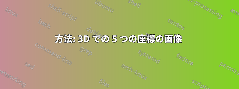
出力は次のようになります。

という数値を定義したことに注意してください\rot。その値を(たとえば)30まで変更すると、自動的に別の視点が得られます。さらに、奥行きをもっと出したい場合は、破線を描くこともできます。奥行きが足りないのは主にy座標の小さな変化によるものなので、その方向のスケールを変更することもできます。たとえば、y={((-\rot:3cm))}

上記のコードに次の数行を追加するだけです (\def\rot{30}前文に注意してください)。
\begin{tikzpicture}[x={(180+\rot:1cm)},y={(-\rot:3cm)},z={(90:1cm)},...]
...
\draw [dashed] (pt1)--+(0,-1,0) (pt1)--+(0,0,-10);
\draw [dashed] (pt2)--+(0,0,-9) (pt2)--+(-9,0,0);
\draw [dashed] (pt3)--+(0,-2,0) (pt3)--+(0,0,-1);
\draw [dashed] (pt4)--+(-8,0,0) (pt4)--+(0,-2,0);
...
\end{tikzpicture}