3D交差点

Question

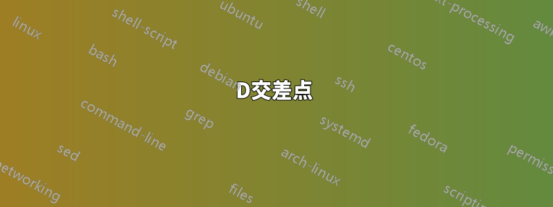
練習として、プリズム[0,2] x [0,4] x [0,6]と平面x + y + z = 5の交点を描いてみます。

私の結果は次のとおりです:

\documentclass{article}

\usepackage{pgfplots}
\pgfplotsset{compat=newest}

\begin{document}
    
\begin{tikzpicture}[x={(-0.45cm,-0.385cm)},y={(1cm,-0.1cm)},z={(0,1cm)}]
    \draw [->] (0,0,0) -- (6,0,0) node [below left] {$x$};
    \draw [->] (0,0,0) -- (0,6,0) node [right] {$y$};
    \draw [->] (0,0,0) -- (0,0,6) node [right] {$z$};
    
    \filldraw [thick, orange, fill opacity=0.3] (0,0,5) -- (0,4,1) -- (1,4,0) -- (2,3,0) -- (2,0,3) -- cycle;
    \filldraw [thick, blue, fill opacity=0.2] (2,3,0) -- (2,0,3) -- (5,0,0) -- cycle;
    \filldraw [thick, blue, fill opacity=0.2] (1,4,0) -- (0,5,0) -- (0,4,1) -- cycle;
    
    \filldraw [thick, orange, fill opacity=0.3] (2,3,0) -- (2,0,0) -- (2,0,3) -- cycle;
    \filldraw [thick, orange, fill opacity=0.3] (1,4,0) -- (0,4,0) -- (0,4,1) --cycle;
    
\end{tikzpicture}

\end{document}

いくつか質問があります:

• 簡単な数学的な体積を [0,2] x [0,4] x [0,6] として表すだけでも、多くのコードが必要になると思います。もっと効率的に描画する方法はありますか?
• 交差を手作業で計算して表現する必要がありますか? それとも直接的な方法がありますか?
• の代わりにaxis環境とコマンドを使用して同じ結果を得るにはどうすればよいですか? 試してみましたが、初心者なので軸の位置 ( ) で問題があり、色が均一ではなく、表面には画像の理解を困難にするグリッドがあり、交差点についても同じ疑問があります。手動で計算する必要がありますか?\addplot\draw\addplot3view={}{}colormap

フルプリズムとは:

\draw [fill=orange, fill opacity=0.3] (0,0,6) -- (2,0,6) -- (2,4,6) -- (0,4,6) -- cycle ;
\draw [fill=orange, fill opacity=0.3] (2,0,0) -- (2,0,6) -- (2,4,6) -- (2,4,0) -- cycle ;
\draw [fill=orange, fill opacity=0.3] (2,4,0) -- (0,4,0) -- (0,4,6) -- (2,4,6) -- cycle ;

Answer 1

何をするにしても、3Dビューをより体系的にインストールすることを検討してください。おそらく、これを実現する最良の方法はasymptote、3Dで交差を計算するツールを備えた を使用することです。 を使用する場合はpgfplots、 を使用してくださいpatch plots。ただし、この場合も交差を自分で計算する必要があります。この投稿では、実験的なTiけZライブラリこれにより、3D での交差を計算することもできます。

\documentclass{article}
\usepackage{tikz}
\usetikzlibrary{3dtools}%https://github.com/marmotghost/tikz-3dtools
\begin{document}
\pgfdeclarelayer{background} 
\pgfdeclarelayer{foreground}
\pgfdeclarelayer{behind}  
\pgfsetlayers{behind,background,main,foreground}   
\begin{tikzpicture}[>=stealth,
    3d/install view={theta=70,phi=110},
    line cap=round,line join=round,
    visible/.style={draw,thick,solid},
    hidden/.style={draw,very thin,cheating dash},
    3d/polyhedron/.cd,fore/.style={visible,fill opacity=0.6},
    back/.style={fill opacity=0.6,hidden,3d/polyhedron/complete dashes},
    fore layer=foreground,
    back layer=background
    ]
  \draw [->] (0,0,0) coordinate (O) -- (6,0,0) coordinate (ex) node [below left] {$x$};
  \draw [->] (0,0,0) -- (0,6,0) coordinate (ey) node [right] {$y$};
  \draw [->] (0,0,0) -- (0,0,6) coordinate (ez) node [right] {$z$};
  \path (5,0,0) coordinate (A) (0,5,0) coordinate (B) (0,0,5) coordinate (C)
   (2.5,0,0) coordinate (a) (0,3.5,0) coordinate (b) (0,0,2) coordinate (c) ;
  \path[3d/.cd,plane with normal={(ex) through (a) named px},
      plane with normal={(ey) through (b) named py},
      line through={(A) and (B) named lAB},
      line through={(A) and (C) named lAC},
      line through={(B) and (C) named lBC}];
  \path[3d/intersection of={lAB with px}] coordinate (pABx)
   [3d/intersection of={lAB with py}] coordinate (pABy)
   [3d/intersection of={lAC with px}] coordinate (pACx)
   [3d/intersection of={lBC with py}] coordinate (pBCy);
  \pgfmathsetmacro{\mybarycenterA}{barycenter("(A),(pABx),(pACx),(a)")} 
  \pgfmathsetmacro{\mybarycenterB}{barycenter("(B),(pABy),(pBCy),(b)")} 
  \tikzset{3d/polyhedron/.cd,O={(\mybarycenterA)},color=blue,
      draw face with corners={{(A)},{(pABx)},{(pACx)}},
      draw face with corners={{(A)},{(pABx)},{(a)}},
      draw face with corners={{(A)},{(a)},{(pACx)}},
      O={(\mybarycenterB)},
      draw face with corners={{(B)},{(pABy)},{(pBCy)}},
      draw face with corners={{(B)},{(pABy)},{(b)}},
      draw face with corners={{(B)},{(b)},{(pBCy)}},
      color=orange,O={(1,1,1)},
      draw face with corners={{(pABx)},{(pACx)},{(C)},{(pBCy)},{(pABy)}},
      draw face with corners={{(a)},{(pACx)},{(C)},{(O)}},
      draw face with corners={{(b)},{(pBCy)},{(C)},{(O)}},
      draw face with corners={{(b)},{(pABy)},{(pABx)},{(a)},{(O)}}
      }
\end{tikzpicture}
\end{document}

まだ多くの努力が必要です。しかし、1つの利点があります。ビューを変更しても正しい結果が得られます。たとえば3d/install view={theta=70,phi=60},、

もちろん、これはasymptoteおよびpatch plotソリューションにも当てはまります (おそらく、隠れた線を自動的に破線にする可能性を除いて)。