


下のグラフに、方程式 x+y-30 を持つ半透明の垂直の赤い区切り線を追加します。曲線を 2 つのセクションに分割する必要があります。

\documentclass[border=10pt]{standalone}
\usepackage{pgfplots}
\usepgfplotslibrary{fillbetween}
\pgfplotsset{compat=1.17}
\begin{document}
    \begin{tikzpicture}
        \begin{axis} [
            xtick = {0,20,...,100},
            ytick = {0,20,...,60},
            ztick = {0,40,...,120},
            xlabel = $U_A$, ylabel = $U_B$, zlabel = $S$,
            zlabel style={rotate=-90},
            ticklabel style = {font = \scriptsize},
            colormap/cool
            ]
            \addplot3[name path=toppath, domain=0:30, fill=blue, opacity=0.1, fill opacity=0.4,samples=30] (x,30-x,120);
            \addplot3[name path=botpath, domain=0:30, fill=blue, opacity=0.1, fill opacity=0.4,samples=30] (x,30-x,0);
            \addplot [red] fill between[of=toppath and botpath];
            \addplot3 [surf, shader=interp, domain=0:100, domain y=0:60, samples=56]
            { ln((100!/(x!*(100-x)!))*(60!/(y!*(60-y)!))) };
        \end{axis}
    \end{tikzpicture}
\end{document}
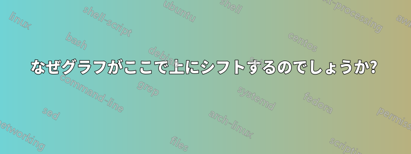
コードを実行すると、奇妙な結果が出ました

元の曲線がなぜ上方にシフトするのか理解できません。
私が見たいのはこれだ

(また、ビューを変更する最適な方法は何ですか。表示ボックスの左隅の視点からグラフを見たいです。)
答え1
残念ながら、この種のオーバーレイは ではまだ利用できませんpgfplots。唯一の解決策は、サーフェスのさまざまな部分、この場合は交差する平面を、正しく重なるように正しい順序で別々にプロットすることです。長方形以外の領域に関数をプロットするには、使用する領域をパラメーター化する必要があります。この場合、上から見ると、三角形と多角形があります。

頂点を指定して三角形をパラメータ化するのは簡単ですが、多角形の場合は複雑になることがあります。最も簡単な解決策は、多角形を追加の三角形に分割することだと思います。

3 つの頂点、が与えられた三角形をパラメータ化するには、次のパラメータ化を使用できます。
値を取得したら、すべてのサーフェスをプロットして完全なサーフェスを取得できます。また、サンプリング レートを高く設定する必要があります。そうしないと、低品質のレンダリングによるエッジの不規則性により、部分的なサーフェスの接合部間にギャップが生じます。これは非常に要求の厳しいソリューションであるため、以下にコードとオプションを使用した結果のグラフを示しshell-escapeますgnuplot。
のみ使用pgfplots:
\documentclass[border=10pt]{standalone}

\usepackage{pgfplots}
\pgfplotsset{compat=newest}

\begin{document}

    \begin{tikzpicture}
        \begin{axis} [
            xtick = {0,20,...,100},
            ytick = {0,20,...,60},
            ztick = {0,40,...,120},
            xlabel = $U_A$, ylabel = $U_B$, zlabel = $S$,
            zlabel style={rotate=-90},
            ticklabel style = {font = \scriptsize},
            colormap/cool,
            variable=s,
            variable y=t,
            domain=0:1,
            view/h=15,
            ]
\addplot3 [surf, shader=interp, samples=80, samples y=80] ({100-100*s},{-30*s-30*t*s+60},{ ln((100!/(x!*(100-x)!))*(60!/(y!*(60-y)!))) }); %B

\addplot3 [surf,shader=interp, samples=30, samples y=30,] ({100*t*s+30-30*s},{30*s+30*t*s},{ ln((100!/(x!*(100-x)!))*(60!/(y!*(60-y)!))) }); %C

\addplot3 [surf, shader=interp, samples=30, samples y=30,] ({100+70*t*s-70*s},{60*t*s},{ ln((100!/(x!*(100-x)!))*(60!/(y!*(60-y)!))) }); %D

\addplot3 [patch, fill=red, patch type=rectangle] coordinates {(0,30,120) (30,0,120)  (30,0,0) (0,30,0)};

\addplot3 [surf, shader=interp, samples=30, samples y=30] ({30-30*s},{30*s*t},{  ln((100!/(x!*(100-x)!))*(60!/(y!*(60-y)!))) }); %A

       \end{axis}
    \end{tikzpicture}

\end{document}

pgfplotsと の使用gnuplot:
\documentclass[border=10pt, convert={true}]{standalone}

\usepackage{pgfplots}
\pgfplotsset{compat=newest}

\begin{document}

    \begin{tikzpicture}
        \begin{axis} [
            xtick = {0,20,...,100},
            ytick = {0,20,...,60},
            ztick = {0,40,...,120},
            xlabel = $U_A$, ylabel = $U_B$, zlabel = $S$,
            zlabel style={rotate=-90},
            ticklabel style = {font = \scriptsize},
            colormap/cool,
            view/h=15,
            ]

           \addplot3[surf, shader=interp, thick ]  gnuplot [ raw gnuplot, id=B ]  {
           set samples 60,60;
           set isosamples 60,60;
           set parametric;
           fx(u,v)=100-100*u;
           fy(u,v)=-30*u-30*v*u+60;
           fz(u,v)= log((100!/((int((100-100*u)))!*(100-int((100-100*u)))!))*(60!/((int((-30*u-30*v*u+60)))!*(60-int((-30*u-30*v*u+60)))!)));
           splot [0:1][0:1] fx(u,v), fy(u,v), fz(u,v)}; %B

            \addplot3[surf, shader=interp]  gnuplot [ raw gnuplot, id=C]  {
           set samples 60,60;
           set isosamples 60,60;
           set parametric;
           gx(u,v)=100*v*u+30-30*u;
           gy(u,v)=30*u+30*v*u;
           gz(u,v)= log((100!/((int(100*v*u+30-30*u))!*(100-int(100*v*u+30-30*u))!))*(60!/((int(30*u+30*v*u))!*(60-int(30*u+30*v*u))!)));
           splot [0:1][0:1] gx(u,v), gy(u,v), gz(u,v) }; %C

           \addplot3[surf, shader=interp]  gnuplot [ raw gnuplot, id=D]  {
    set samples 60,60;
    set isosamples 60,60;
           set parametric;
           hx(u,v)=100+70*v*u-70*u;
           hy(u,v)= 60*v*u;
           hz(u,v)=log((100!/((int(100+70*v*u-70*u))!*(100-int(100+70*v*u-70*u))!))*(60!/((int(60*v*u))!*(60-int(60*v*u))!)));
           splot [0:1][0:1] hx(u,v), hy(u,v), hz(u,v) }; %D

                        \addplot3 [patch, fill=red, patch type=rectangle] coordinates {(0,30,120) (30,0,120)  (30,0,0) (0,30,0)};

                        \addplot3[surf, shader=interp]  gnuplot [raw gnuplot, id=A ]  {
                        set samples 60,60;
                        set isosamples 60,60;
                        set parametric;
                        splot [0:1][0:1] 30-30*u,30*u*v,log((100!/((int(30-30*u))!*(100-int(30-30*u))!))*(60!/((int(30*u*v))!*(60-int(30*u*v))!)))   }; %A


       \end{axis}
    \end{tikzpicture}

\end{document}

ビューを変更するには、view/h= angleオプションを使用できます。適切な重なりを実現するために、サーフェスの順序を適切に調整することを忘れないでください。
2 つの方法のレンダリングにはいくつかの違いがあります。より良い結果を得ることはできませんでしたが、サンプリングを調整して、より良い組み合わせを見つけられるかどうか試してみてください。