


曲線を表示するコードを作成しました。コードは次のとおりです。
\documentclass[12pt]{article}
\usepackage{pgfplots}
\usepackage{amsmath}
\pgfplotsset{compat=1.18}
\usepackage{xcolor}
\begin{document}
\pgfplotstableread[col sep=comma]{
-1.00000000e+00, 1.00000000e+00, -3.50000000e+00, 9.75000000e+00, -2.62500000e+01, 7.35937500e+01, -3.50000000e+00, 9.75000000e+00, -2.62500000e+01, 1.23005515e+02
-5.78947368e-01, 1.00000000e+00, -3.07894737e+00, 6.97991690e+00, -1.45631652e+01, 3.17518749e+01, -3.07894737e+00, 6.97991690e+00, -1.45631652e+01, 5.91648918e+01
-1.57894737e-01, 1.00000000e+00, -2.65789474e+00, 4.56440443e+00, -6.15144336e+00, 7.79163062e+00, -2.65789474e+00, 4.56440443e+00, -6.15144336e+00, 1.93708181e+01
2.63157895e-01, 1.00000000e+00, -2.23684211e+00, 2.50346260e+00, -5.66955824e-01, -3.42580172e+00, -2.23684211e+00, 2.50346260e+00, -5.66955824e-01, -2.35859076e+00
6.84210526e-01, 1.00000000e+00, -1.81578947e+00, 7.97091413e-01, 2.63817612e+00, -6.28491883e+00, -1.81578947e+00, 7.97091413e-01, 2.63817612e+00, -1.12508974e+01
1.10526316e+00, 1.00000000e+00, -1.39473684e+00, -5.54709141e-01, 3.91183117e+00, -4.41589541e+00, -1.39473684e+00, -5.54709141e-01, 3.91183117e+00, -1.17793423e+01
1.52631579e+00, 1.00000000e+00, -9.73684211e-01, -1.55193906e+00, 3.70188803e+00, -6.94584190e-01, -9.73684211e-01, -1.55193906e+00, 3.70188803e+00, -7.66284401e+00
1.94736842e+00, 1.00000000e+00, -5.52631579e-01, -2.19459834e+00, 2.45622540e+00, 2.75748416e+00, -5.52631579e-01, -2.19459834e+00, 2.45622540e+00, -1.86599894e+00
2.36842105e+00, 1.00000000e+00, -1.31578947e-01, -2.48268698e+00, 6.22721971e-01, 4.57310099e+00, -1.31578947e-01, -2.48268698e+00, 6.22721971e-01, 3.40091845e+00
2.78947368e+00, 1.00000000e+00, 2.89473684e-01, -2.41620499e+00, -1.35074355e+00, 4.13937964e+00, 2.89473684e-01, -2.41620499e+00, -1.35074355e+00, 6.68195573e+00
3.21052632e+00, 1.00000000e+00, 7.10526316e-01, -1.99515235e+00, -3.01629246e+00, 1.59775549e+00, 7.10526316e-01, -1.99515235e+00, -3.01629246e+00, 7.27548248e+00
3.63157895e+00, 1.00000000e+00, 1.13157895e+00, -1.21952909e+00, -3.92604607e+00, -2.15601404e+00, 1.13157895e+00, -1.21952909e+00, -3.92604607e+00, 5.23419032e+00
4.05263158e+00, 1.00000000e+00, 1.55263158e+00, -8.93351801e-02, -3.63212567e+00, -5.47184956e+00, 1.55263158e+00, -8.93351801e-02, -3.63212567e+00, 1.36509289e+00
4.47368421e+00, 1.00000000e+00, 1.97368421e+00, 1.39542936e+00, -1.68665257e+00, -5.94534961e+00, 1.97368421e+00, 1.39542936e+00, -1.68665257e+00, -2.77047418e+00
4.89473684e+00, 1.00000000e+00, 2.39473684e+00, 3.23476454e+00, 2.35825193e+00, -4.17790734e-01, 2.39473684e+00, 3.23476454e+00, 2.35825193e+00, -4.85685319e+00
5.31578947e+00, 1.00000000e+00, 2.81578947e+00, 5.42867036e+00, 8.95046654e+00, 1.50238725e+01, 2.81578947e+00, 5.42867036e+00, 8.95046654e+00, -1.82406447e+00
5.73684211e+00, 1.00000000e+00, 3.23684211e+00, 7.97714681e+00, 1.85378700e+01, 4.50470077e+01, 3.23684211e+00, 7.97714681e+00, 1.85378700e+01, 1.01521937e+01
6.15789474e+00, 1.00000000e+00, 3.65789474e+00, 1.08801939e+01, 3.15683409e+01, 9.50733043e+01, 3.65789474e+00, 1.08801939e+01, 3.15683409e+01, 3.56505451e+01
6.57894737e+00, 1.00000000e+00, 4.07894737e+00, 1.41378116e+01, 4.84897580e+01, 1.71278774e+02, 4.07894737e+00, 1.41378116e+01, 4.84897580e+01, 8.00039353e+01
7.00000000e+00, 1.00000000e+00, 4.50000000e+00, 1.77500000e+01, 6.97500000e+01, 2.80593750e+02, 4.50000000e+00, 1.77500000e+01, 6.97500000e+01, 1.49299632e+02
}\loadedtable
\begin{figure}[h]
\tikzset{ellipsenode/.style={draw, ellipse, thick, text width=5ex, align=center, inner sep=2pt}}
\begin{tikzpicture}
\begin{axis}[
axis lines=center,
xmin=-0.6, xmax=6.6,
ymin=-17, ymax=28,
axis on top,
xtick distance=1,
ytick distance=5,
tick label style={font=\footnotesize, inner sep=1pt, fill=white},
no marks, samples=15, smooth,
legend entries={
$Q^{1/2,1/2,5}_{0}(x)$,
$Q^{1/2,1/2,5}_{1}(x)$,
$Q^{1/2,1/2,5}_{2}(x)$,
$Q^{1/2,1/2,5}_{3}(x)$,
$Q^{1/2,1/2,5}_{4}(x)$
}, ]
\addplot[color=red] table[x index=0,y index=1] {\loadedtable};
\addplot[color=blue]table[x index=0,y index=2] {\loadedtable};
\addplot[color=green] table[x index=0,y index=3] {\loadedtable};
\addplot[color=purple] table[x index=0,y index=4] {\loadedtable};
\addplot[color=yellow] table[x index=0,y index=5] {\loadedtable};
\end{axis}
\end{tikzpicture}
\begin{tikzpicture}
\begin{axis}[
axis lines=center,
xmin=-0.6, xmax=6.6,
ymin=-17, ymax=28,
axis on top,
xtick distance=1,
ytick distance=5,
tick label style={font=\footnotesize, inner sep=1pt, fill=white},
no marks, samples=15, smooth,
legend entries={
$Q^{(3)}_{0}(x)$,
$Q^{(3)}_{1}(x)$,
$Q^{(3)}_{2}(x)$,
$Q^{(3)}_{3}(x)$,
$Q^{(3)}_{4}(x)$
},
]
\addplot[color=red] table[x index=0,y index=1] {\loadedtable};
\addplot[color=blue]table[x index=0,y index=6] {\loadedtable};
\addplot[color=green] table[x index=0,y index=7] {\loadedtable};
\addplot[color=purple] table[x index=0,y index=8] {\loadedtable};
\addplot[color=yellow] table[x index=0,y index=9] {\loadedtable};
\end{axis}
\end{tikzpicture}
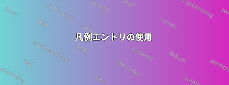
\caption{Graph of $Q^{1/2,1/2,5}_n$ and $Q^{(3)}_n$ for $n = 0, 1, 2, 3, 4$}
\end{figure}
\end{document}
結果

しかし、コンパイル結果では、2つの説明テーブルを小さくしてグラフを見やすくしたいです。アイデアをお願いします
答え1
に関して。リンク付きの私のコメント独自の凡例をデザインまたはタイプセットする方法を次に示します。違いをよりよく確認し、混乱を避けるために、別の回答として記載しました。

備考
前文
standaloneデザインには、必要に応じて「紙」のサイズに調整されるクラスを使用する方が適しています。パッケージはここでは必要ありません。凡例をタイプセットするには、xcolortikzlibrary が必要になります。matrix
\documentclass[10pt,border=3mm,tikz]{standalone}
\usepackage{pgfplots}
\usepackage{amsmath}
\pgfplotsset{compat=1.18}
%\usepackage{xcolor}    % <<< not needed in pgfplots
\usetikzlibrary{matrix} % <<< to typeset the legend, later
プロットセット
組み込みの凡例は使用しないため、これは廃止されています。
%    \pgfplotsset{
%       every axis legend/.append style={
%           at={(1.02,1)},
%           anchor=north west,
%       },
%    }
軸環境
- タイトルをつけましょう
- すべての凡例文を削除する
\labelそれぞれに後を追加\addplot ... ;\coordinate後で使用するために定義します。ここでは(label)
    \begin{axis}[
        ...
        no marks, samples=15, smooth,
        title=$Q^{1/2,1/2,5}_n(x)$; % <<<
    ]
    % <<< new: put labels, to reference them later ~~~~~~~~~~~~~~~~~~~~~~~~~~~~~~
    \addplot[color=red] table[x index=0,y index=1] {\loadedtable};\label{plot:L1}
    ...

    % <<< new: legend will go here, in plot coordinates
    \coordinate (legend) at (.3,25);
    \end{axis}
凡例をタイプセットする
基本的な構造は で\matrix[...] at (legend) { ... };、 の場合とほぼ同じです\node。 希望どおりに表示するには、いくつかのスタイルを定義する必要があります。
\matrixを の Tikz ペンダントとして考えてくださいLatex table。1 行のデータの構造が表示されるのはそのためです& & \\。内部では、通常のテキストと同じようにタイプセットし、以前に設定したすべてのプロット ラベルを参照します。すべての参照と同様に、変更を加えた後は 2 回目のコンパイルが必要です。
    % ~~~ building your legend using a matrix (it's like a table within Tikz) ~~~~
    \matrix[
        draw,               % to see it, with
        matrix of nodes,    % see manual
        anchor=north west,  % upper left corner
        font={\tiny},       % use smaller font, if you like
    ] at (legend) {
        Index $n$: &&\\
        \ref{plot:L1} 0&\ref{plot:L2} 1&\ref{plot:L3} 2\\
        \ref{plot:L4} 3&\ref{plot:L5} 4&\\
    };
結果とコード

\documentclass[10pt,border=3mm,tikz]{standalone}
\usepackage{pgfplots}
\usepackage{amsmath}
\pgfplotsset{compat=1.18}
%\usepackage{xcolor}    % <<< not needed in pgfplots
\usetikzlibrary{matrix} % <<< to typeset the legend, later

% ~~~~~~~~~~~~~~~~~~~~~~~~~~~~~~~~~~~
\begin{document}
    \pgfplotstableread[col sep=comma]{
           -1.00000000e+00,  1.00000000e+00, -3.50000000e+00,         9.75000000e+00, -2.62500000e+01,  7.35937500e+01, -3.50000000e+00,         9.75000000e+00, -2.62500000e+01,  1.23005515e+02
           -5.78947368e-01,  1.00000000e+00, -3.07894737e+00,         6.97991690e+00, -1.45631652e+01,  3.17518749e+01, -3.07894737e+00,         6.97991690e+00, -1.45631652e+01,  5.91648918e+01
           -1.57894737e-01,  1.00000000e+00, -2.65789474e+00,         4.56440443e+00, -6.15144336e+00,  7.79163062e+00, -2.65789474e+00,         4.56440443e+00, -6.15144336e+00,  1.93708181e+01
            2.63157895e-01,  1.00000000e+00, -2.23684211e+00,         2.50346260e+00, -5.66955824e-01, -3.42580172e+00, -2.23684211e+00,         2.50346260e+00, -5.66955824e-01, -2.35859076e+00
            6.84210526e-01,  1.00000000e+00, -1.81578947e+00,         7.97091413e-01,  2.63817612e+00, -6.28491883e+00, -1.81578947e+00,         7.97091413e-01,  2.63817612e+00, -1.12508974e+01
            1.10526316e+00,  1.00000000e+00, -1.39473684e+00,        -5.54709141e-01,  3.91183117e+00, -4.41589541e+00, -1.39473684e+00,        -5.54709141e-01,  3.91183117e+00, -1.17793423e+01
            1.52631579e+00,  1.00000000e+00, -9.73684211e-01,        -1.55193906e+00,  3.70188803e+00, -6.94584190e-01, -9.73684211e-01,        -1.55193906e+00,  3.70188803e+00, -7.66284401e+00
            1.94736842e+00,  1.00000000e+00, -5.52631579e-01,        -2.19459834e+00,  2.45622540e+00,  2.75748416e+00, -5.52631579e-01,        -2.19459834e+00,  2.45622540e+00, -1.86599894e+00
            2.36842105e+00,  1.00000000e+00, -1.31578947e-01,        -2.48268698e+00,  6.22721971e-01,  4.57310099e+00, -1.31578947e-01,        -2.48268698e+00,  6.22721971e-01,  3.40091845e+00
            2.78947368e+00,  1.00000000e+00,  2.89473684e-01,        -2.41620499e+00, -1.35074355e+00,  4.13937964e+00,  2.89473684e-01,        -2.41620499e+00, -1.35074355e+00,  6.68195573e+00
            3.21052632e+00,  1.00000000e+00,  7.10526316e-01,        -1.99515235e+00, -3.01629246e+00,  1.59775549e+00,  7.10526316e-01,        -1.99515235e+00, -3.01629246e+00,  7.27548248e+00
            3.63157895e+00,  1.00000000e+00,  1.13157895e+00,        -1.21952909e+00, -3.92604607e+00, -2.15601404e+00,  1.13157895e+00,        -1.21952909e+00, -3.92604607e+00,  5.23419032e+00
            4.05263158e+00,  1.00000000e+00,  1.55263158e+00,        -8.93351801e-02, -3.63212567e+00, -5.47184956e+00,  1.55263158e+00,        -8.93351801e-02, -3.63212567e+00,  1.36509289e+00
            4.47368421e+00,  1.00000000e+00,  1.97368421e+00,         1.39542936e+00, -1.68665257e+00, -5.94534961e+00,  1.97368421e+00,         1.39542936e+00, -1.68665257e+00, -2.77047418e+00
            4.89473684e+00,  1.00000000e+00,  2.39473684e+00,         3.23476454e+00,  2.35825193e+00, -4.17790734e-01,  2.39473684e+00,         3.23476454e+00,  2.35825193e+00, -4.85685319e+00
            5.31578947e+00,  1.00000000e+00,  2.81578947e+00,         5.42867036e+00,  8.95046654e+00,  1.50238725e+01,  2.81578947e+00,         5.42867036e+00,  8.95046654e+00, -1.82406447e+00
            5.73684211e+00,  1.00000000e+00,  3.23684211e+00,         7.97714681e+00,  1.85378700e+01,  4.50470077e+01,  3.23684211e+00,         7.97714681e+00,  1.85378700e+01,  1.01521937e+01
            6.15789474e+00,  1.00000000e+00,  3.65789474e+00,         1.08801939e+01,  3.15683409e+01,  9.50733043e+01,  3.65789474e+00,         1.08801939e+01,  3.15683409e+01,  3.56505451e+01
            6.57894737e+00,  1.00000000e+00,  4.07894737e+00,         1.41378116e+01,  4.84897580e+01,  1.71278774e+02,  4.07894737e+00,         1.41378116e+01,  4.84897580e+01,  8.00039353e+01
            7.00000000e+00,  1.00000000e+00,  4.50000000e+00,         1.77500000e+01,  6.97500000e+01,  2.80593750e+02,  4.50000000e+00,         1.77500000e+01,  6.97500000e+01,  1.49299632e+02

}\loadedtable

\tikzset{
    ellipsenode/.style={
        draw, ellipse, thick, text width=5ex,
        align=center, inner sep=2pt
    }
}

    \begin{tikzpicture}
%    \pgfplotsset{
%       every axis legend/.append style={
%           at={(1.02,1)},
%           anchor=north west,
%       },
%    }
    \begin{axis}[
        axis lines=center,
        xmin=-0.6,  xmax=6.6,
        ymin=-17,  ymax=28,
        axis on top,
        xtick distance=1,
        ytick distance=5,
        tick label style={font=\footnotesize, inner sep=1pt, fill=white},
        no marks, samples=15, smooth,
        title=$Q^{1/2,1/2,5}_n(x)$; % <<<
    ]
    % <<< new: put labels, to reference them later ~~~~~~~~~~~~~~~~~~~~~~~~~~~~~~
    \addplot[color=red] table[x index=0,y index=1] {\loadedtable};\label{plot:L1}
    \addplot[color=blue]table[x index=0,y index=2] {\loadedtable};\label{plot:L2}
    \addplot[color=green] table[x index=0,y index=3] {\loadedtable};\label{plot:L3}
    \addplot[color=purple] table[x index=0,y index=4] {\loadedtable};\label{plot:L4}
    \addplot[color=yellow] table[x index=0,y index=5] {\loadedtable};\label{plot:L5}

    % <<< new: legend will go here, in plot coordinates
    \coordinate (legend) at (.3,25);
    \end{axis}

    % ~~~ building your legend using a matrix (it's like a table within Tikz) ~~~~
    \matrix[
        draw,               % to see it, with
        matrix of nodes,    % see manual
        anchor=north west,  % upper left corner
        font={\tiny},       % use smaller font, if you like
    ] at (legend) {
        Index $n$: &&\\
        \ref{plot:L1} 0&\ref{plot:L2} 1&\ref{plot:L3} 2\\
        \ref{plot:L4} 3&\ref{plot:L5} 4&\\
    };
    \end{tikzpicture}
\end{document}
答え2
これを行う 1 つの方法は次のとおりです。最も簡単な方法は、凡例を図面の外側、たとえば右側に配置することです。「4.9.5 凡例の外観」(pdf)または「20.9 凡例の外観」(html)pgfplots マニュアルで説明されています。
上に凡例を配置してみましたが、見栄えがよくありません。また、この章の最初のページで説明されている方法を使用して、独自の凡例を Tikz で描画することもできます。
% from said chapter, sth. like this:
 \matrix [style=every axis legend] {
    draw plot specification 1 & \node{legend 1}\\
...
もう一つの選択肢は、記事で多くの機能の略語を導入し、それをグラフで使用することです。略語が短い場合は、投稿したように 2 つの図を 1 行のグラフとしてまとめることができます。
あなたのコードとの違いは、私が両方のプロットに追加した次のコード行です。
- 軸の凡例のスタイルを指定する
- マニュアルにあるように、(0,0)は左下、(1,1)は右上隅です。
- 凡例を右上に少しずらして配置する
- 左上隅(
north west)を上記の位置に固定する
\begin{tikzpicture}
\pgfplotsset{                                 % <<<
    every axis legend/.append style={
        at={(1.02,1)},
        anchor=north west
    },
}
\begin{axis}[

% https://tex.stackexchange.com/questions/705129/using-legend-entries

\documentclass[12pt]{article}
\usepackage{pgfplots}
\usepackage{amsmath}
\pgfplotsset{compat=1.18}
\usepackage{xcolor}
\begin{document}
\pgfplotstableread[col sep=comma]{
       -1.00000000e+00,  1.00000000e+00, -3.50000000e+00,         9.75000000e+00, -2.62500000e+01,  7.35937500e+01, -3.50000000e+00,         9.75000000e+00, -2.62500000e+01,  1.23005515e+02
       -5.78947368e-01,  1.00000000e+00, -3.07894737e+00,         6.97991690e+00, -1.45631652e+01,  3.17518749e+01, -3.07894737e+00,         6.97991690e+00, -1.45631652e+01,  5.91648918e+01
       -1.57894737e-01,  1.00000000e+00, -2.65789474e+00,         4.56440443e+00, -6.15144336e+00,  7.79163062e+00, -2.65789474e+00,         4.56440443e+00, -6.15144336e+00,  1.93708181e+01
        2.63157895e-01,  1.00000000e+00, -2.23684211e+00,         2.50346260e+00, -5.66955824e-01, -3.42580172e+00, -2.23684211e+00,         2.50346260e+00, -5.66955824e-01, -2.35859076e+00
        6.84210526e-01,  1.00000000e+00, -1.81578947e+00,         7.97091413e-01,  2.63817612e+00, -6.28491883e+00, -1.81578947e+00,         7.97091413e-01,  2.63817612e+00, -1.12508974e+01
        1.10526316e+00,  1.00000000e+00, -1.39473684e+00,        -5.54709141e-01,  3.91183117e+00, -4.41589541e+00, -1.39473684e+00,        -5.54709141e-01,  3.91183117e+00, -1.17793423e+01
        1.52631579e+00,  1.00000000e+00, -9.73684211e-01,        -1.55193906e+00,  3.70188803e+00, -6.94584190e-01, -9.73684211e-01,        -1.55193906e+00,  3.70188803e+00, -7.66284401e+00
        1.94736842e+00,  1.00000000e+00, -5.52631579e-01,        -2.19459834e+00,  2.45622540e+00,  2.75748416e+00, -5.52631579e-01,        -2.19459834e+00,  2.45622540e+00, -1.86599894e+00
        2.36842105e+00,  1.00000000e+00, -1.31578947e-01,        -2.48268698e+00,  6.22721971e-01,  4.57310099e+00, -1.31578947e-01,        -2.48268698e+00,  6.22721971e-01,  3.40091845e+00
        2.78947368e+00,  1.00000000e+00,  2.89473684e-01,        -2.41620499e+00, -1.35074355e+00,  4.13937964e+00,  2.89473684e-01,        -2.41620499e+00, -1.35074355e+00,  6.68195573e+00
        3.21052632e+00,  1.00000000e+00,  7.10526316e-01,        -1.99515235e+00, -3.01629246e+00,  1.59775549e+00,  7.10526316e-01,        -1.99515235e+00, -3.01629246e+00,  7.27548248e+00
        3.63157895e+00,  1.00000000e+00,  1.13157895e+00,        -1.21952909e+00, -3.92604607e+00, -2.15601404e+00,  1.13157895e+00,        -1.21952909e+00, -3.92604607e+00,  5.23419032e+00
        4.05263158e+00,  1.00000000e+00,  1.55263158e+00,        -8.93351801e-02, -3.63212567e+00, -5.47184956e+00,  1.55263158e+00,        -8.93351801e-02, -3.63212567e+00,  1.36509289e+00
        4.47368421e+00,  1.00000000e+00,  1.97368421e+00,         1.39542936e+00, -1.68665257e+00, -5.94534961e+00,  1.97368421e+00,         1.39542936e+00, -1.68665257e+00, -2.77047418e+00
        4.89473684e+00,  1.00000000e+00,  2.39473684e+00,         3.23476454e+00,  2.35825193e+00, -4.17790734e-01,  2.39473684e+00,         3.23476454e+00,  2.35825193e+00, -4.85685319e+00
        5.31578947e+00,  1.00000000e+00,  2.81578947e+00,         5.42867036e+00,  8.95046654e+00,  1.50238725e+01,  2.81578947e+00,         5.42867036e+00,  8.95046654e+00, -1.82406447e+00
        5.73684211e+00,  1.00000000e+00,  3.23684211e+00,         7.97714681e+00,  1.85378700e+01,  4.50470077e+01,  3.23684211e+00,         7.97714681e+00,  1.85378700e+01,  1.01521937e+01
        6.15789474e+00,  1.00000000e+00,  3.65789474e+00,         1.08801939e+01,  3.15683409e+01,  9.50733043e+01,  3.65789474e+00,         1.08801939e+01,  3.15683409e+01,  3.56505451e+01
        6.57894737e+00,  1.00000000e+00,  4.07894737e+00,         1.41378116e+01,  4.84897580e+01,  1.71278774e+02,  4.07894737e+00,         1.41378116e+01,  4.84897580e+01,  8.00039353e+01
        7.00000000e+00,  1.00000000e+00,  4.50000000e+00,         1.77500000e+01,  6.97500000e+01,  2.80593750e+02,  4.50000000e+00,         1.77500000e+01,  6.97500000e+01,  1.49299632e+02

}\loadedtable
\begin{figure}[h]
\tikzset{ellipsenode/.style={draw, ellipse, thick, text width=5ex, align=center, inner sep=2pt}}
\begin{tikzpicture}
\pgfplotsset{
    every axis legend/.append style={
        at={(1.02,1)},
        anchor=north west
    },
}
\begin{axis}[
axis lines=center,
xmin=-0.6,  xmax=6.6,
ymin=-17,  ymax=28,
axis on top,
xtick distance=1,
ytick distance=5,
tick label style={font=\footnotesize, inner sep=1pt, fill=white},
no marks, samples=15, smooth,
legend entries={
        $Q^{1/2,1/2,5}_{0}(x)$,
        $Q^{1/2,1/2,5}_{1}(x)$,
        $Q^{1/2,1/2,5}_{2}(x)$,
        $Q^{1/2,1/2,5}_{3}(x)$,
        $Q^{1/2,1/2,5}_{4}(x)$
},                ]
\addplot[color=red] table[x index=0,y index=1] {\loadedtable};
\addplot[color=blue]table[x index=0,y index=2] {\loadedtable};
\addplot[color=green] table[x index=0,y index=3] {\loadedtable};
\addplot[color=purple] table[x index=0,y index=4] {\loadedtable};
\addplot[color=yellow] table[x index=0,y index=5] {\loadedtable};
\end{axis}
\end{tikzpicture}
% ~~~~~~~~~~~~~~~~~~~~~~~~~~~
\begin{tikzpicture}
\pgfplotsset{
    every axis legend/.append style={
        at={(1.02,1)},
        anchor=north west
    },
}
\begin{axis}[
axis lines=center,
xmin=-0.6,  xmax=6.6,
ymin=-17,  ymax=28,
axis on top,
xtick distance=1,
ytick distance=5,
tick label style={font=\footnotesize, inner sep=1pt, fill=white},
no marks, samples=15, smooth,
legend entries={
        $Q^{(3)}_{0}(x)$,
        $Q^{(3)}_{1}(x)$,
        $Q^{(3)}_{2}(x)$,
        $Q^{(3)}_{3}(x)$,
        $Q^{(3)}_{4}(x)$
},
   ]
\addplot[color=red] table[x index=0,y index=1] {\loadedtable};
\addplot[color=blue]table[x index=0,y index=6] {\loadedtable};
\addplot[color=green] table[x index=0,y index=7] {\loadedtable};
\addplot[color=purple] table[x index=0,y index=8] {\loadedtable};
\addplot[color=yellow] table[x index=0,y index=9] {\loadedtable};
\end{axis}
\end{tikzpicture}
\caption{Graph of $Q^{1/2,1/2,5}_n$ and $Q^{(3)}_n$ for $n = 0, 1, 2, 3, 4$}
\end{figure}
\end{document}
追伸:
参考までに、凡例をプロットの上部に移動すると次のようになります。

両方に を使用します:
\pgfplotsset{
    every axis legend/.append style={
        at={(.5,1.03)},
        anchor=south
    },
}
追伸2
title次は、 を使用して関連する変更のみに焦点を当てた別の方法です: n。ただし、0、1、... のみをリストしても、ここでは凡例が十分に小さくなりません。

\begin{axis}[
    axis lines=center,
    xmin=-0.6,  xmax=6.6,
    ymin=-17,  ymax=28,
    axis on top,
    xtick distance=1,
    ytick distance=5,
    tick label style={font=\footnotesize, inner sep=1pt, fill=white},
    no marks, samples=15, smooth,
    legend entries={
            $n=0$,              % <<<
            $n=1$,
            $n=2$,
            $n=3$,
            $n=4$,
    },
    title=$Q^{1/2,1/2,5}_n(x)$; % <<<
]