離散整数値のヒストグラム

Question

タイトルの通り、整数値からヒストグラムを作成したいと思います。私の MWE は次のとおりです。

\documentclass[border=5]{standalone}

\usepackage{pgfplots}
%Random data between 10 and 20 -- could also be between 100 and 200 or what ever
\begin{filecontents*}{data.txt}
        18
        15
        18
        19
        14
        15
        12
        11
        18
        18
        12
        11
        17
\end{filecontents*}

\begin{document}
    \begin{tikzpicture}
        \begin{axis}[
            axis lines=left,
            ymajorgrids=true,
            title={Histogram},
            xlabel=points,
            ylabel=headcount,
            ybar
            ]
        \addplot+ [hist] table[y index= 0]{data.txt};
        \end{axis}
    \end{tikzpicture}
\end{document}

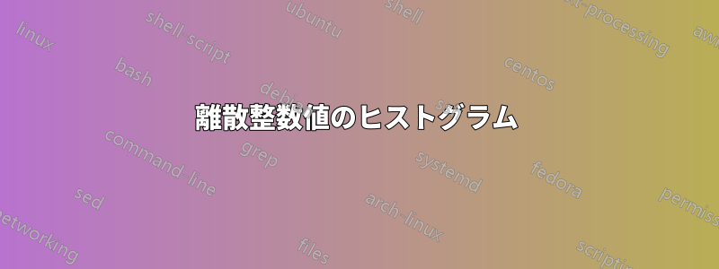
結果は次のとおりです。

私が得たいのは次のものです (注: 残念ながら、値を二重にカウントしてしまいました):

問題は、x 軸が離散的ではないため、ラベルがずれてしまうことです。バーの間にスペースを設けたいのですが、y 軸と最初のバーの間、および最後のバーにもスペースを設けたいです。

追加情報: 私は LaTeX を使用しています。すでに精度を 0 に設定し、データツールを使用して最初に頻度をカウントしてから、簡単な棒グラフを描画しようとしました。さまざまなラベルとエリアのスタイルに苦労しましたが、目標を達成できませんでした。

Answer 1

gnuplot を使用してヒストグラム データを作成し、これらのデータを棒グラフとしてプロットすることができます。コンパイルするには、gnuplot をインストールし、次のコマンドでコンパイルする必要があります--shell-escape。--shell-escape は何をしますか?

\begin{filecontents*}{data.txt}
18
15
18
19
14
15
12
11
18
18
12
11
17
\end{filecontents*}
\documentclass[tikz, border=1cm]{standalone}
\usepackage{pgfplots}
\pgfplotsset{compat=1.18}
\begin{document}
\begin{tikzpicture}
\begin{axis}[
ybar,
xmin=10, xmax=20,
ymin=0,
xtick distance=1,
axis lines=left,
ymajorgrids=true,
title={Not a Histogram}, xlabel=points, ylabel=headcount,
]
\addplot+[raw gnuplot] gnuplot {
binwidth=1;
bin(x,bw)=bw*floor(x/bw);
plot "data.txt" using (bin($1,binwidth)):(1.0) smooth freq;
};
\end{axis}
\end{tikzpicture}
\end{document}

Answer 2

• Latex3ランダムに選択したデータも準備できます。

  \intarray_new:Nn \g_HISTO_myarray_intarray {9}

1から9までの数字（11、12、...、19を除く）を保存します。ファイルに書き込むときに10を追加します。\jobname.data

• すでにファイルの準備ができている場合、またはデータを手動で変更する場合は、このファイルを変更してコメントすることができます\histo[20]。

• とpgfplots

  bar width=0.5cmenlarge x limits={auto},enlarge y limits={upper},軸に固執しないように

コード

\documentclass[border=5mm]{standalone}
\usepackage{pgfplots}
\pgfplotsset{compat=1.18}
\ExplSyntaxOn
%%%%%%%%%%%%%%%%%%%%%%%%%%%
\sys_gset_rand_seed:n {240210}
%%%%%%%%%%%%%%%%%%%%%%%%%%%
\int_new:N \l_HISTO_randominteger_int
\intarray_new:Nn \g_HISTO_myarray_intarray {9}
\iow_new:N \g_HISTO_iow
%
\tl_new:N \l_HISTO_table_tl
\NewDocumentCommand{\histo}{O{10}}% 10 by default
    {
        \__array_fillarray:n{#1}       
        \__array_table:       
    }

\cs_new_protected:Nn \__array_fillarray:n
{
    \int_step_inline:nnn {1} {#1} 
            {
                \int_set:Nn \l_HISTO_randominteger_int {\int_rand:nn {1} {9}}
                \intarray_gset:Nnn \g_HISTO_myarray_intarray 
                    { \l_HISTO_randominteger_int } 
                    { 
                        \intarray_item:Nn \g_HISTO_myarray_intarray {\l_HISTO_randominteger_int} + 1
                    }
                %\int_use:N \l_HISTO_randominteger_int \quad % uncomment to see the numbers
            }
    %\intarray_log:N \g_HISTO_myarray_intarray% <-- to see the intarray in the log
}

\cs_new_protected:Nn \__array_table:
    {
        \iow_open:Nn \g_HISTO_iow {\jobname.data}
        \int_step_inline:nnn {1} {9}
            {
                \tl_clear:N \l_HISTO_table_tl
                \tl_put_right:Nn \l_HISTO_table_tl {\int_eval:n {10+##1}}%<-- between 11 and 19
                \tl_put_right:Nn \l_HISTO_table_tl {~}
                \tl_put_right:Nn \l_HISTO_table_tl {
                \intarray_item:Nn \g_HISTO_myarray_intarray {##1}}         
                \iow_now:Nx \g_HISTO_iow { \l_HISTO_table_tl }
            }
        \iow_close:N \g_HISTO_iow 
    }
\ExplSyntaxOff
\begin{document}
\histo[20]

\begin{tikzpicture}
    \begin{axis}[
        %width=8cm, height=8cm,
        axis lines=left,
        ybar,
        bar width=0.5cm,
        ymajorgrids=true,
        title={Histogram ?},%<-- ?
        %
        xlabel=points,
        ylabel=headcount,
        xticklabel style = {font=\small},
        xtick=data,
        enlarge x limits={auto},
        enlarge y limits={upper},
    ]
    \addplot table[y index=1]  {\jobname.data};
    \end{axis}
\end{tikzpicture}
\end{document}