


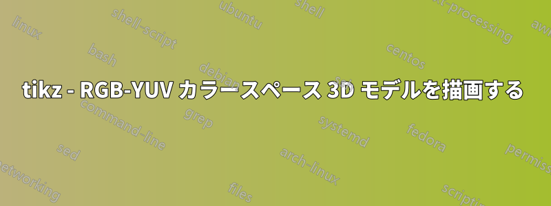
3D RGB-YUV カラー スペース モデルを描画したいと思います。これは次のようになります。

RGB キューブ カラー スペース (0,255)、RGB から YUV への変換式は次のとおりです。

YUV から RGB への変換式:

数式に示されたとおりの正確なグラフを取得したいのですが、このような図を描くにはどのパッケージの方が適しているでしょうか?
答え1
はい、Tiに教えることはできますけZ を使用して線形変換を行います。スクリーンショットには非正投影が表示されています。そのため、個人的にはあまり好きではありませんが、回答の最後にそのような投影を追加します。RGBvec線形変換を行う関数を追加します (特に、これらの情報がどこから来ているかわからない場合は、画面からテキストを入力するのが得意ではないため、タイプミスは除きます)。また、RGB 座標を他の配色に変換するクイック スタイルを追加しました。これらすべてを調整できますが、少なくともこれは、原理的にはこれをどのように実行できるかを示しています。
\documentclass[tikz,border=3mm]{standalone}
\usepackage{tikz-3dplot}
\def\matCC{{0.257, 0.504, 0.098},%
        {-0.148, -0.291, 0.439},%
        {0.439, -0.368,0.071}}%
\pgfmathdeclarefunction{RGBvec}{3}{%
\begingroup%
\pgfmathsetmacro{\myY}{16+{\matCC}[0][0]*#1+{\matCC}[0][1]*#2+{\matCC}[0][2]*#3}%
\pgfmathsetmacro{\myCb}{128+{\matCC}[1][0]*#1+{\matCC}[1][1]*#2+{\matCC}[1][2]*#3}%
\pgfmathsetmacro{\myCr}{128+{\matCC}[2][0]*#1+{\matCC}[2][1]*#2+{\matCC}[2][2]*#3}%
\edef\pgfmathresult{\myCr,\myCb,\myY}%
\pgfmathsmuggle\pgfmathresult\endgroup%
}%

\begin{document}
\tdplotsetmaincoords{70}{110}
\begin{tikzpicture}[bullet/.style={circle,inner
    sep=2pt,fill},line cap=round,line join=round,
    RGB coordinate/.code args={(#1,#2,#3)}{\pgfmathparse{RGBvec(#1,#2,#3)}%
    \tikzset{insert path={(\pgfmathresult)}}},font=\sffamily,thick]
 \begin{scope}[tdplot_main_coords,scale=1/40]
  \draw[-stealth] (0,0,0) coordinate (O) -- (280,0,0) coordinate[label=below:Cr] (Cr);
  \draw[-stealth]  (O) -- (0,280,0) coordinate[label=below:Cb] (Cb);
  \draw[-stealth]  (O) -- (0,0,280) coordinate[label=left:Y] (Y);
  \path [RGB coordinate={(255,255,255)}] node[bullet,draw,fill=white] (white){}
    [RGB coordinate={(0,0,0)}] node[bullet] (black){}
    [RGB coordinate={(255,0,0)}] node[bullet,red] (red){}
    [RGB coordinate={(0,255,0)}] node[bullet,green] (green){}
    [RGB coordinate={(0,0,255)}] node[bullet,blue] (blue){}
    [RGB coordinate={(255,0,255)}] node[bullet,magenta] (magenta){}
    [RGB coordinate={(255,255,0)}] node[bullet,yellow] (yellow){}
    [RGB coordinate={(0,255,255)}] node[bullet,cyan] (cyan){};
   \draw (red) -- (black) -- (blue) -- (magenta) -- (red) -- (yellow)
   -- (green) edge (black) -- (cyan) edge (blue) -- (white)  edge (magenta) -- (yellow);
   \draw[thin] (255,0,0) node[left]{255} -- (255,255,0) -- (0,255,0) node[above]{255}
   (0,0,255) node[left]{255} -- (255,0,255) edge (255,0,0)
    -- (255,255,255)  edge (255,255,0) -- (0,255,255)  edge (0,255,0)
   -- cycle ;
 \end{scope}
 \begin{scope}[xshift=8cm,scale=1/40]
  \pgfmathdeclarefunction*{RGBvec}{3}{%
  \begingroup%
  \pgfmathsetmacro{\myY}{16+{\matCC}[0][0]*#1+{\matCC}[0][1]*#2+{\matCC}[0][2]*#3}%
  \pgfmathsetmacro{\myCb}{128+{\matCC}[1][0]*#1+{\matCC}[1][1]*#2+{\matCC}[1][2]*#3}%
  \pgfmathsetmacro{\myCr}{128+{\matCC}[2][0]*#1+{\matCC}[2][1]*#2+{\matCC}[2][2]*#3}%
  \edef\pgfmathresult{\myCb,\myY,\myCr}%
  \pgfmathsmuggle\pgfmathresult\endgroup%
  }%
  \draw[-stealth] (0,0,0) coordinate (O) -- (255,0,0) coordinate[label=below:Cb] (Cb);
  \draw[-stealth]  (O) -- (0,255,0) coordinate[label=left:Y] (Y);
  \draw[-stealth]  (O) -- (0,0,255) coordinate[label=below:Cr] (Cr);
  \path [RGB coordinate={(255,255,255)}] node[bullet,draw,fill=white] (white){}
    [RGB coordinate={(0,0,0)}] node[bullet] (black){}
    [RGB coordinate={(255,0,0)}] node[bullet,red] (red){}
    [RGB coordinate={(0,255,0)}] node[bullet,green] (green){}
    [RGB coordinate={(0,0,255)}] node[bullet,blue] (blue){}
    [RGB coordinate={(255,0,255)}] node[bullet,magenta] (magenta){}
    [RGB coordinate={(255,255,0)}] node[bullet,yellow] (yellow){}
    [RGB coordinate={(0,255,255)}] node[bullet,cyan] (cyan){};
   \draw (red) -- (black) -- (blue) -- (magenta) -- (red) -- (yellow)
   -- (green) edge (black) -- (cyan) edge (blue) -- (white)  edge (magenta) -- (yellow);
  \end{scope}
\end{tikzpicture}
\end{document}

正投影の利点は、直交変換、つまり回転を適用でき、結果がリアルになることです (遠近法の効果まで、ライブラリを使用して処理できますperspective)。
\documentclass[tikz,border=3mm]{standalone}
\usepackage{tikz-3dplot}
\def\matCC{{0.257, 0.504, 0.098},%
        {-0.148, -0.291, 0.439},%
        {0.439, -0.368,0.071}}%
\pgfmathdeclarefunction{RGBvec}{3}{%
\begingroup%
\pgfmathsetmacro{\myY}{16+{\matCC}[0][0]*#1+{\matCC}[0][1]*#2+{\matCC}[0][2]*#3}%
\pgfmathsetmacro{\myCb}{128+{\matCC}[1][0]*#1+{\matCC}[1][1]*#2+{\matCC}[1][2]*#3}%
\pgfmathsetmacro{\myCr}{128+{\matCC}[2][0]*#1+{\matCC}[2][1]*#2+{\matCC}[2][2]*#3}%
\edef\pgfmathresult{\myCr,\myCb,\myY}%
\pgfmathsmuggle\pgfmathresult\endgroup%
}%
\tikzset{RGB coordinate/.code args={(#1,#2,#3)}{\pgfmathparse{RGBvec(#1,#2,#3)}%
    \tikzset{insert path={(\pgfmathresult)}}}}
\begin{document}
\foreach \X in {0,10,...,350}
{\tdplotsetmaincoords{70}{\X}
\begin{tikzpicture}[bullet/.style={circle,inner
    sep=2pt,fill},line cap=round,line join=round,font=\sffamily,thick]
 \path[use as bounding box] (-5.5,-2)   rectangle (5.5,8);
 \begin{scope}[tdplot_main_coords,scale=1/40,shift={(-128,-128,0)}]
  \draw[-stealth] (0,0,0) coordinate (O) -- (280,0,0) coordinate[label=below:Cr] (Cr);
  \draw[-stealth]  (O) -- (0,280,0) coordinate[label=below:Cb] (Cb);
  \draw[-stealth]  (O) -- (0,0,280) coordinate[label=left:Y] (Y);
  \path [RGB coordinate={(255,255,255)}] node[bullet,draw,fill=white] (white){}
    [RGB coordinate={(0,0,0)}] node[bullet] (black){}
    [RGB coordinate={(255,0,0)}] node[bullet,red] (red){}
    [RGB coordinate={(0,255,0)}] node[bullet,green] (green){}
    [RGB coordinate={(0,0,255)}] node[bullet,blue] (blue){}
    [RGB coordinate={(255,0,255)}] node[bullet,magenta] (magenta){}
    [RGB coordinate={(255,255,0)}] node[bullet,yellow] (yellow){}
    [RGB coordinate={(0,255,255)}] node[bullet,cyan] (cyan){};
   \draw (red) -- (black) -- (blue) -- (magenta) -- (red) -- (yellow)
   -- (green) edge (black) -- (cyan) edge (blue) -- (white)  edge (magenta) -- (yellow);
   \draw[thin] (255,255,0) -- (255,0,0) node[pos=1.1]{255}
   (255,255,0) --(0,255,0) node[pos=1.1]{255}
   (0,0,255) node[left]{255} -- (255,0,255) edge (255,0,0)
    -- (255,255,255)  edge (255,255,0) -- (0,255,255)  edge (0,255,0)
   -- cycle ;
 \end{scope}
\end{tikzpicture}}
\end{document}

もちろん、接続部分に色の変化を表現することもできます。
\documentclass[tikz,border=3mm]{standalone}
\usepackage{tikz-3dplot}
\def\matCC{{0.257, 0.504, 0.098},%
        {-0.148, -0.291, 0.439},%
        {0.439, -0.368,0.071}}%
\pgfmathdeclarefunction{RGBvec}{3}{%
\begingroup%
\pgfmathsetmacro{\myY}{16+{\matCC}[0][0]*#1+{\matCC}[0][1]*#2+{\matCC}[0][2]*#3}%
\pgfmathsetmacro{\myCb}{128+{\matCC}[1][0]*#1+{\matCC}[1][1]*#2+{\matCC}[1][2]*#3}%
\pgfmathsetmacro{\myCr}{128+{\matCC}[2][0]*#1+{\matCC}[2][1]*#2+{\matCC}[2][2]*#3}%
\edef\pgfmathresult{\myCr,\myCb,\myY}%
\pgfmathsmuggle\pgfmathresult\endgroup%
}%
\tikzset{RGB coordinate/.code args={(#1,#2,#3)}{\pgfmathparse{RGBvec(#1,#2,#3)}%
    \tikzset{insert path={(\pgfmathresult)}}}}
\begin{document}
\tdplotsetmaincoords{70}{110}
\begin{tikzpicture}[bullet/.style={circle,inner
    sep=2pt,outer sep=0pt,fill},connection bar/.style args={(#1)--(#2)}{%
    insert path={let \p1=(#1),\p2=(#2),\n1={atan2(\y2-\y1,\x2-\x1)} in
    [left color=#1,right color=#2,shading angle=\n1+90]
    (#1.\n1-25) arc(\n1-25:\n1+25:40*2pt)
    -- (#2.\n1-180-25)  arc(\n1-180-25:\n1-180+25:40*2pt) -- cycle}},
    line cap=round,line join=round,font=\sffamily,thick]
 \path[use as bounding box] (-5.5,-2)   rectangle (5.5,8);
 \begin{scope}[tdplot_main_coords,scale=1/40,shift={(-128,-128,0)}]
  \draw[-stealth] (0,0,0) coordinate (O) -- (280,0,0) coordinate[label=below:Cr] (Cr);
  \draw[-stealth]  (O) -- (0,280,0) coordinate[label=below:Cb] (Cb);
  \draw[-stealth]  (O) -- (0,0,280) coordinate[label=left:Y] (Y);
  \path [RGB coordinate={(255,255,255)}] node[bullet,draw,fill=white] (white){}
    [RGB coordinate={(0,0,0)}] node[bullet] (black){}
    [RGB coordinate={(255,0,0)}] node[bullet,red] (red){}
    [RGB coordinate={(0,255,0)}] node[bullet,green] (green){}
    [RGB coordinate={(0,0,255)}] node[bullet,blue] (blue){}
    [RGB coordinate={(255,0,255)}] node[bullet,magenta] (magenta){}
    [RGB coordinate={(255,255,0)}] node[bullet,yellow] (yellow){}
    [RGB coordinate={(0,255,255)}] node[bullet,cyan] (cyan){};
  \path[connection bar={(black)--(blue)}];
  \path[connection bar={(blue)--(magenta)}];
  \path[connection bar={(magenta)--(red)}];
  \path[connection bar={(red)--(black)}];
  \path[connection bar={(white)--(magenta)}];
  \path[connection bar={(cyan)--(blue)}];
  \path[connection bar={(green)--(black)}];
  \path[connection bar={(yellow)--(red)}];
  \path[connection bar={(yellow)--(green)}];
  \path[connection bar={(green)--(cyan) }];
  \path[connection bar={(cyan)--(white)}];
  \path[connection bar={(white)--(yellow)}];
   \draw[thin] (255,255,0) -- (255,0,0) node[pos=1.1]{255}
   (255,255,0) --(0,255,0) node[pos=1.1]{255}
   (0,0,255) node[left]{255} -- (255,0,255) edge (255,0,0)
    -- (255,255,255)  edge (255,255,0) -- (0,255,255)  edge (0,255,0)
   -- cycle ;
 \end{scope}
\end{tikzpicture}
\end{document}

いくつかのコメント:
- 原理的には、線形変換を行うには、はるかに簡単な方法があります。
\begin{scope}[x={(x)},y={(y)},x={(y)}] ... \end{scope}、ここで(x)、(y)および は(z)基底ベクトルです。ただし、シフトが追加されると少し混乱するので、座標を明示的に指定した方がよいと考えました。 \pgfshadecolortorgbRGB 座標で色を変換できます。この投稿を書いているときは、これを使用することは考えていませんでした。
答え2
出発点です。これで 3D 座標上に描画できます。あなたのプロフィールを見ると、それができると思います。
\documentclass[tikz,margin=3]{standalone}
\usetikzlibrary{arrows.meta}
\begin{document}
\begin{tikzpicture}[z={(-135:.5)},>=Stealth]
  \draw[thick,->] (0,0,0) -- (5,0,0) node[below] {Cb};
  \draw[thick,->] (0,0,0) -- (0,5,0) node[left] {Y};
  \draw[thick,->] (0,0,0) -- (0,0,5) node[below] {Cr};
  \draw (4,0,0) node[anchor=135] {255} |- (0,4,0) node[anchor=-30] {255}
    -- (0,4,4) |- (4,0,4) -- cycle
    (0,4,4) -| (4,0,4) (4,4,4) -- (4,4,0)
    (0,0,4) node[anchor=-30] {255};
  \path (0,0) node[below] {0};
\end{tikzpicture}
\end{document}
