


Ich habe versucht, ein Tikz-Bild zu erstellen, das 5 Punkte in 3D darstellt, wobei von einem Punkt 4 Vektoren zu den anderen 4 Punkten ausgehen. Ich frage mich, ob es eine Möglichkeit gibt, dieses Bild dreidimensional aussehen zu lassen.
\documentclass[landscape]{article}
\usepackage{tikz}
\usepackage{verbatim}
\usepackage[active,tightpage]{preview}
\PreviewEnvironment{tikzpicture}
\setlength\PreviewBorder{10pt}%
\usetikzlibrary{calc}


\begin{document}
\begin{tikzpicture}
[
scale=3,
>=stealth,
point/.style = {draw, circle,  fill = black, inner sep = 1pt},
dot/.style   = {draw, circle,  fill = black, inner sep = .2pt},
]

%% Vanishing points for perspective handling
\coordinate (P1) at (-9cm,1.5cm); % left vanishing point (To pick)
\coordinate (P2) at (9cm,1.5cm); % right vanishing point (To pick)

%% (A1) and (A2) defines the 2 central points of the cuboid
\coordinate (A1) at (0em,3cm); % central top point (To pick)
\coordinate (A2) at (0em,-3cm); % central bottom point (To pick)

%% (A3) to (A8) are computed given a unique parameter (or 2) .8
% You can vary .8 from 0 to 1 to change perspective on left side
\coordinate (A3) at ($(P1)!.8!(A2)$); % To pick for perspective
\coordinate (A4) at ($(P1)!.8!(A1)$);

% You can vary .8 from 0 to 1 to change perspective on right side
\coordinate (A7) at ($(P2)!.7!(A2)$);
\coordinate (A8) at ($(P2)!.7!(A1)$);

%% Automatically compute the last 2 points with intersections
\coordinate (A5) at
  (intersection cs: first line={(A8) -- (P1)},
            second line={(A4) -- (P2)});
\coordinate (A6) at
  (intersection cs: first line={(A7) -- (P1)},
            second line={(A3) -- (P2)});


%% Possibly draw back faces
\fill[gray!90] (A2) -- (A3) -- (A6) -- (A7) -- cycle; % face 6
\node at (barycentric cs:A2=1,A3=1,A6=1,A7=1) {\tiny };
\fill[gray!50] (A3) -- (A4) -- (A5) -- (A6) -- cycle; % face 3
\node at (barycentric cs:A3=1,A4=1,A5=1,A6=1) {\tiny };
\fill[gray!30] (A5) -- (A6) -- (A7) -- (A8) -- cycle; % face 4
\node at (barycentric cs:A5=1,A6=1,A7=1,A8=1) {\tiny };

\draw[thick] (A5) -- (A6);
\draw[thick] (A3) -- (A6);
\draw[thick] (A7) -- (A6);

\node (n0) at (0,0) [point, label = left:$S$] {};
\node (n1) at (1.2,1.7) [point, label = left:$R_{1}$] {};
\node (n2) at (-0.5, 1.2) [point, label = left:$R_{2}$] {};
\node (n3) at (1.35,-1.1) [point, label = left:$R_{3}$] {};
\node (n4) at (-0.2, -1.9) [point, label = left:$R_{4}$] {};

\draw[<-] (n1) -- node (a) [label = {below right:$d_{1}$}] {} (n0);
\draw[<-] (n2) -- node (b) [label = {above right:$d_{2}$}] {} (n0);
\draw[<-] (n3) -- node (c) [label = {above right:$d_{3}$}] {} (n0);
\draw[<-] (n4) -- node (d) [label = {above right:$d_{4}$}] {} (n0);

\end{tikzpicture}
\end{document}

Antwort1
Wenn Sie nicht wirklich in 3D zeichnen möchten, was möglich ist mittikz-3dplotPaket, dann ist eine sehr einfache Lösung, die Flächen mit einigen sehr hellen Farben zu füllen. Siehe das Bild unten.

Dies ist der Code für Ihren Fall
\documentclass[landscape]{article}
\usepackage{tikz}
\usepackage{verbatim}
\usepackage[active,tightpage]{preview}
\PreviewEnvironment{tikzpicture}
\setlength\PreviewBorder{10pt}%
\usetikzlibrary{calc}


\begin{document}
\begin{tikzpicture}
[
scale=3,
>=stealth,
point/.style = {draw, circle,  fill = black, inner sep = 1pt},
dot/.style   = {draw, circle,  fill = black, inner sep = .2pt},
]

%% Vanishing points for perspective handling
\coordinate (P1) at (-9cm,1.5cm); % left vanishing point (To pick)
\coordinate (P2) at (9cm,1.5cm); % right vanishing point (To pick)

%% (A1) and (A2) defines the 2 central points of the cuboid
\coordinate (A1) at (0em,3cm); % central top point (To pick)
\coordinate (A2) at (0em,-3cm); % central bottom point (To pick)

%% (A3) to (A8) are computed given a unique parameter (or 2) .8
% You can vary .8 from 0 to 1 to change perspective on left side
\coordinate (A3) at ($(P1)!.8!(A2)$); % To pick for perspective
\coordinate (A4) at ($(P1)!.8!(A1)$);

% You can vary .8 from 0 to 1 to change perspective on right side
\coordinate (A7) at ($(P2)!.7!(A2)$);
\coordinate (A8) at ($(P2)!.7!(A1)$);

%% Automatically compute the last 2 points with intersections
\coordinate (A5) at
  (intersection cs: first line={(A8) -- (P1)},
            second line={(A4) -- (P2)});
\coordinate (A6) at
  (intersection cs: first line={(A7) -- (P1)},
            second line={(A3) -- (P2)});


%% Possibly draw back faces
\fill[gray!90] (A2) -- (A3) -- (A6) -- (A7) -- cycle; % face 6
\node at (barycentric cs:A2=1,A3=1,A6=1,A7=1) {\tiny };
\fill[gray!50] (A3) -- (A4) -- (A5) -- (A6) -- cycle; % face 3
\node at (barycentric cs:A3=1,A4=1,A5=1,A6=1) {\tiny };
\fill[gray!30] (A5) -- (A6) -- (A7) -- (A8) -- cycle; % face 4
\node at (barycentric cs:A5=1,A6=1,A7=1,A8=1) {\tiny };

\draw[thick] (A5) -- (A6);
\draw[thick] (A3) -- (A6);
\draw[thick] (A7) -- (A6);

\node (n0) at (0,0) [point, label = left:$S$] {};
\node (n1) at (1.2,1.7) [point, label = left:$R_{1}$] {};
\node (n2) at (-0.5, 1.2) [point, label = left:$R_{2}$] {};
\node (n3) at (1.35,-1.1) [point, label = left:$R_{3}$] {};
\node (n4) at (-0.2, -1.9) [point, label = left:$R_{4}$] {};


\draw[fill, green, opacity=.1] (0,0) -- (1.2,1.7) -- (-0.5, 1.2);
\draw[fill, green, opacity=.1] (0,0) -- (-0.2, -1.9) -- (1.35,-1.1);
\draw[fill, red, opacity=.05] (0,0) -- (1.2,1.7) -- (1.35,-1.1);


\draw[<-,very thick] (n1) -- node (a) [label = {below right:$d_{1}$}] {} (n0);
\draw[<-,very thick] (n2) -- node (b) [label = {above right:$d_{2}$}] {} (n0);
\draw[<-,very thick] (n3) -- node (c) [label = {above right:$d_{3}$}] {} (n0);
\draw[<-,very thick] (n4) -- node (d) [label = {above right:$d_{4}$}] {} (n0);


\end{tikzpicture}
\end{document}
Antwort2
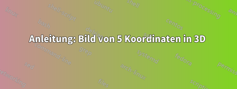
Ich würde die in Ti verfügbaren Koordinatentransformationsmakros verwendenkZ, die es grundsätzlich ermöglichen, einen neuen Satz von Koordinaten x, y und z als Funktion des „alten“ Systems u, v zu definieren, wie unten gezeigt:

Ich finde diesen Code weniger knifflig und mit weniger Berechnungen verbunden:
\documentclass[tikz,convert]{standalone}
\begin{document}
\def\rot{30}
\begin{tikzpicture}[x={(180+\rot:1cm)},y={(-\rot:1cm)},z={(90:1cm)},scale=.7,>=stealth,thick]


\draw [fill=gray,draw=none] (0,0,0)--(10,0,0)--(10,5,0)--(0,5,0)--cycle;
\draw [fill=gray!50!white,draw=none] (0,0,0)--(10,0,0)--(10,0,15)--(0,0,15)--cycle;
\draw [fill=gray!30!white,draw=none] (0,0,0)--(0,5,0)--(0,5,15)--(0,0,15)--cycle;
\draw (0,0,0)--(10,0,0) (0,0,0)--(0,5,0) (0,0,0)--(0,0,15);


\node [fill=black,circle,inner sep=1pt] (pt0) at (5,0.5,5) {};
\node [fill=black,circle,inner sep=1pt] (pt1) at (0,1,10) {};
\node [fill=black,circle,inner sep=1pt] (pt2) at (9,0,9) {};
\node [fill=black,circle,inner sep=1pt] (pt3) at (0,2,1) {};
\node [fill=black,circle,inner sep=1pt] (pt4) at (8,2,0) {};

\draw [->] (pt0)--(pt1) node [pos=.5,right] {$d_1$};
\draw [->] (pt0)--(pt2) node [pos=.5,right] {$d_2$};
\draw [->] (pt0)--(pt3) node [pos=.5,below] {$d_3$};
\draw [->] (pt0)--(pt4) node [pos=.5,right] {$d_4$};

\node at (pt0) [left] {$S$};
\node at (pt1) [above] {$R1$};
\node at (pt2) [left] {$R2$};
\node at (pt3) [right] {$R3$};
\node at (pt4) [below] {$R4$};
\end{tikzpicture}
\end{document}
und dies ist die Ausgabe:

Beachten Sie, dass ich eine Zahl namens definiert habe \rot. Wenn Sie ihren Wert auf beispielsweise 30 ändern, erhalten Sie automatisch eine andere Perspektive. Wenn Sie außerdem mehr Tiefe wünschen, können Sie auch gestrichelte Linien zeichnen. Da der Mangel an Tiefe hauptsächlich auf die kleinen Änderungen der Y-Koordinate zurückzuführen ist, können Sie auch den Maßstab dieser Richtung ändern, beispielsweisey={((-\rot:3cm))}

indem Sie dem obigen Code einfach diese paar Zeilen hinzufügen (Hinweis \def\rot{30}in der Präambel):
\begin{tikzpicture}[x={(180+\rot:1cm)},y={(-\rot:3cm)},z={(90:1cm)},...]
...
\draw [dashed] (pt1)--+(0,-1,0) (pt1)--+(0,0,-10);
\draw [dashed] (pt2)--+(0,0,-9) (pt2)--+(-9,0,0);
\draw [dashed] (pt3)--+(0,-2,0) (pt3)--+(0,0,-1);
\draw [dashed] (pt4)--+(-8,0,0) (pt4)--+(0,-2,0);
...
\end{tikzpicture}