Tangential-, Normal- und Binormalvektoren

Question

Ich möchte eine schematische Abbildung zeichnen, die die Koordinatensystembeziehung zwischen dem kartesischen Koordinatensystem und dem natürlichen Helix-Koordinatensystem veranschaulicht. Welche Tools (z. B. tikz-3dplot, Asymptote) eignen sich zum Zeichnen besser?

Answer 1

Ich benutze einige mathematische Formeln sind inHierUndder Frenet-Serret-Rahmen (oder TNB-Rahmen).

Mit den verfügbaren Formeln ist Asymptote-Code schlicht und einfach. Versteckte Linien können gestrichelt werden, aber das gefällt mir nicht, weil sie (T,N,B)dann auch gestrichelt sind ^^

// http://asymptote.ualberta.ca/
unitsize(1cm);
import graph3;
currentprojection=orthographic(3,2,1.5,center=true,zoom=.9);
real a=2;
real h=8;
draw(scale(a,a,h)*unitcylinder,yellow+opacity(.3));
draw(Label("$x$",EndPoint,black),O--4X,gray,Arrow3());
draw(Label("$y$",EndPoint,black),O--4Y,gray,Arrow3());
draw(Label("$z$",EndPoint,black),O--10Z,gray,Arrow3());

triple r(real t){return (a*cos(t),a*sin(t),h*t/(2*pi));}
real tmin=0,tmax=2pi;
path3 g=graph(r,tmin,tmax,operator..);
draw(g,red+.6pt);

triple T(real t){return (-a*sin(t),a*cos(t),h/(2*pi));}
triple N(real t){return (-a*cos(t),-a*sin(t),0);}

pen pentan=purple;
pen pennor=red;
pen penbin=darkgreen;


real t=1;
triple P=r(t);
triple Pt=unit(T(t));         // the tangent vector at P
triple Pn=unit(N(t));         // the normal vector at P
triple Pb=cross(Pt,Pn);       // the binormal vector at P
draw(Label("$T$",EndPoint,pentan),P--P+Pt,pentan,Arrow3);
draw(Label("$N$",EndPoint,pennor),P--P+Pn,pennor,Arrow3);
draw(Label("$B$",EndPoint,penbin),P--P+Pb,penbin,Arrow3);

real s=3;
triple Q=r(s);
triple Qt=unit(T(s));         // the tangent vector at Q
triple Qn=unit(N(s));         // the normal vector at Q
triple Qb=cross(Qt,Qn);       // the binormal vector at Q
draw(Q--Q+Qt,pentan,Arrow3);
draw(Q--Q+Qn,pennor,Arrow3);
draw(Q--Q+Qb,penbin,Arrow3);

real c=4.3;
triple R=r(c);
triple Rt=unit(T(c));         // the tangent vector at R
triple Rn=unit(N(c));         // the normal vector at R
triple Rb=cross(Qt,Qn);       // the binormal vector at R
draw(R--R+Rt,pentan,Arrow3);
draw(R--R+Rn,pennor,Arrow3);
draw(R--R+Rb,penbin,Arrow3);

Answer 2

Ein TikZ-Lösung. Sie verwendet 3dBibliotheken, perspectiveum einige trigonometrische Berechnungen zu vermeiden.

Ich erstelle auch zwei \picS, eines für die Helix und eines für die drei Vektoren. Auf diese Weise können wir beide zeichnen, indem wir nur die beteiligten Winkel aufschreiben.

Der Code:

\documentclass[tikz,border=1.618]{standalone}
\usetikzlibrary{3d,perspective}

\tikzset
{
  surface/.style={draw=cyan,left color=cyan,fill opacity=0.5},
  top/.style={draw=cyan,fill=cyan!30,fill opacity=0.5,canvas is xy plane at z=4},
  pics/helix/.style 2 args={code=% #1 = initial angle, #2 = final angle
    {\draw[pic actions] plot[domain=#1:#2,samples=0.5*#2-0.5*#1+1] ({cos(\x)},{sin(\x)},\x/180);}},
  pics/vectors/.style={code=% #1 = angle
    {\draw[green!50!black,-latex,opacity=0.3] ({cos(#1)},{sin(#1)},#1/180) -- ({0.4*cos(#1)},{0.4*sin(#1)},#1/180) node[pos=1.5] {$\vec N$};
     \begin{scope}[shift={({cos(#1)},{sin(#1)},#1/180)},rotate around z=90+#1,canvas is xz plane at y=0]
       \draw[blue!50!black,-latex]    (0,0) --++ ({atan(1/pi)}:0.75) node[pos=1.4] {$\vec T$};
       \draw[magenta!50!black,-latex] (0,0) --++ ({90+atan(1/pi)}:1) node[pos=1.3] {$\vec B$};
     \end{scope}}}
}

\begin{document}
\begin{tikzpicture}[isometric view,rotate around z=180,font=\small,
                    line cap=round,line join=round]
% axes
\draw[-latex] (0,0,0) -- (2,0,0) node[left]  {\strut$x$};
\draw[-latex] (0,0,0) -- (0,2,0) node[right] {\strut$y$};
% helix,   background
\pic[red] {helix={135}{315}};
\pic[red] {helix={495}{675}};
% z-axis,  background
\draw (0,0,0) -- (0,0,4);
% vectors, background
\foreach\i in {270,550}
  \pic {vectors=\i};
% cylinder
\draw[surface] (-45:1) arc (-45:135:1) --++ (0,0,4) arc (135:-45:1) -- cycle;
\draw[top] (0,0) circle (1);
% z-axis,  foreground
\draw[-latex] (0,0,4) -- (0,0,5.5) node[above] {$z$};
% helix,   foreground
\pic[red] {helix=  {0}{135}};
\pic[red] {helix={315}{495}};
\pic[red] {helix={675}{720}};
% vectors, foreground
\foreach\i in {30,110}
  \pic {vectors=\i};
\end{tikzpicture}
\end{document}

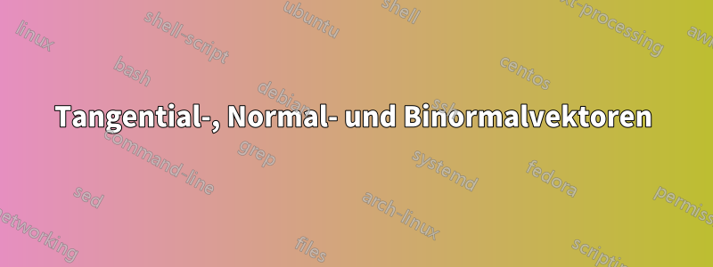
Die Ausgabe: