tikz - RGB-YUV 색상 공간 3D 모델 그리기

Question

3D RGB-YUV 색공간 모델을 그리고 싶습니다. 이는 아래와 같습니다:

RGB 큐브 색상 공간(0,255), RGB에서 YUV로의 변환 공식은 다음과 같습니다.

YUV에서 RGB로 변환 공식:

공식에 명시된 대로 정확한 그래프를 얻고 싶습니다. 그러한 다이어그램을 그리는 데 어떤 패키지가 더 좋을까요?

Answer 1

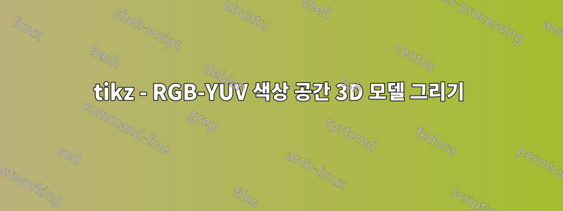
예, Ti를 가르칠 수 있습니다케이Z는 선형 변환을 수행합니다. 스크린샷에는 직교가 아닌 투영이 표시됩니다. 그래서 개인적으로 그다지 좋아하지는 않지만 답변 끝에 그러한 투영을 추가합니다. 선형 변환을 수행하는 기능 RGBvec(특히 화면 쇼에서 텍스트를 입력하는 데 능숙하지 않기 때문에 모듈로 오타)을 추가하고 RGB 좌표를 변환하는 빠른 스타일을 추가했습니다. 다른 색 구성표. 이 모든 것들은 조정될 수 있지만 적어도 이것은 원칙적으로 이것을 어떻게 할 수 있는지를 보여줍니다.

\documentclass[tikz,border=3mm]{standalone}
\usepackage{tikz-3dplot}
\def\matCC{{0.257, 0.504, 0.098},% 
        {-0.148, -0.291, 0.439},%
        {0.439, -0.368,0.071}}%
\pgfmathdeclarefunction{RGBvec}{3}{%
\begingroup%
\pgfmathsetmacro{\myY}{16+{\matCC}[0][0]*#1+{\matCC}[0][1]*#2+{\matCC}[0][2]*#3}%
\pgfmathsetmacro{\myCb}{128+{\matCC}[1][0]*#1+{\matCC}[1][1]*#2+{\matCC}[1][2]*#3}%
\pgfmathsetmacro{\myCr}{128+{\matCC}[2][0]*#1+{\matCC}[2][1]*#2+{\matCC}[2][2]*#3}%
\edef\pgfmathresult{\myCr,\myCb,\myY}%
\pgfmathsmuggle\pgfmathresult\endgroup%
}%

\begin{document}
\tdplotsetmaincoords{70}{110}
\begin{tikzpicture}[bullet/.style={circle,inner
    sep=2pt,fill},line cap=round,line join=round,
    RGB coordinate/.code args={(#1,#2,#3)}{\pgfmathparse{RGBvec(#1,#2,#3)}%
    \tikzset{insert path={(\pgfmathresult)}}},font=\sffamily,thick]
 \begin{scope}[tdplot_main_coords,scale=1/40]
  \draw[-stealth] (0,0,0) coordinate (O) -- (280,0,0) coordinate[label=below:Cr] (Cr);
  \draw[-stealth]  (O) -- (0,280,0) coordinate[label=below:Cb] (Cb);
  \draw[-stealth]  (O) -- (0,0,280) coordinate[label=left:Y] (Y);
  \path [RGB coordinate={(255,255,255)}] node[bullet,draw,fill=white] (white){}
    [RGB coordinate={(0,0,0)}] node[bullet] (black){}
    [RGB coordinate={(255,0,0)}] node[bullet,red] (red){}
    [RGB coordinate={(0,255,0)}] node[bullet,green] (green){}
    [RGB coordinate={(0,0,255)}] node[bullet,blue] (blue){}
    [RGB coordinate={(255,0,255)}] node[bullet,magenta] (magenta){}
    [RGB coordinate={(255,255,0)}] node[bullet,yellow] (yellow){}
    [RGB coordinate={(0,255,255)}] node[bullet,cyan] (cyan){};
   \draw (red) -- (black) -- (blue) -- (magenta) -- (red) -- (yellow) 
   -- (green) edge (black) -- (cyan) edge (blue) -- (white)  edge (magenta) -- (yellow); 
   \draw[thin] (255,0,0) node[left]{255} -- (255,255,0) -- (0,255,0) node[above]{255}
   (0,0,255) node[left]{255} -- (255,0,255) edge (255,0,0)
    -- (255,255,255)  edge (255,255,0) -- (0,255,255)  edge (0,255,0)
   -- cycle ;
 \end{scope}
 \begin{scope}[xshift=8cm,scale=1/40]
  \pgfmathdeclarefunction*{RGBvec}{3}{%
  \begingroup%
  \pgfmathsetmacro{\myY}{16+{\matCC}[0][0]*#1+{\matCC}[0][1]*#2+{\matCC}[0][2]*#3}%
  \pgfmathsetmacro{\myCb}{128+{\matCC}[1][0]*#1+{\matCC}[1][1]*#2+{\matCC}[1][2]*#3}%
  \pgfmathsetmacro{\myCr}{128+{\matCC}[2][0]*#1+{\matCC}[2][1]*#2+{\matCC}[2][2]*#3}%
  \edef\pgfmathresult{\myCb,\myY,\myCr}%
  \pgfmathsmuggle\pgfmathresult\endgroup%
  }%
  \draw[-stealth] (0,0,0) coordinate (O) -- (255,0,0) coordinate[label=below:Cb] (Cb);
  \draw[-stealth]  (O) -- (0,255,0) coordinate[label=left:Y] (Y);
  \draw[-stealth]  (O) -- (0,0,255) coordinate[label=below:Cr] (Cr);
  \path [RGB coordinate={(255,255,255)}] node[bullet,draw,fill=white] (white){}
    [RGB coordinate={(0,0,0)}] node[bullet] (black){}
    [RGB coordinate={(255,0,0)}] node[bullet,red] (red){}
    [RGB coordinate={(0,255,0)}] node[bullet,green] (green){}
    [RGB coordinate={(0,0,255)}] node[bullet,blue] (blue){}
    [RGB coordinate={(255,0,255)}] node[bullet,magenta] (magenta){}
    [RGB coordinate={(255,255,0)}] node[bullet,yellow] (yellow){}
    [RGB coordinate={(0,255,255)}] node[bullet,cyan] (cyan){};
   \draw (red) -- (black) -- (blue) -- (magenta) -- (red) -- (yellow) 
   -- (green) edge (black) -- (cyan) edge (blue) -- (white)  edge (magenta) -- (yellow); 
  \end{scope}   
\end{tikzpicture}
\end{document}

직교 투영에는 직교 변환, 즉 회전을 적용할 수 있고 결과가 사실적이라는 장점이 있습니다(라이브러리를 사용하여 처리할 수 있는 원근 효과까지 perspective).

\documentclass[tikz,border=3mm]{standalone}
\usepackage{tikz-3dplot}
\def\matCC{{0.257, 0.504, 0.098},% 
        {-0.148, -0.291, 0.439},%
        {0.439, -0.368,0.071}}%
\pgfmathdeclarefunction{RGBvec}{3}{%
\begingroup%
\pgfmathsetmacro{\myY}{16+{\matCC}[0][0]*#1+{\matCC}[0][1]*#2+{\matCC}[0][2]*#3}%
\pgfmathsetmacro{\myCb}{128+{\matCC}[1][0]*#1+{\matCC}[1][1]*#2+{\matCC}[1][2]*#3}%
\pgfmathsetmacro{\myCr}{128+{\matCC}[2][0]*#1+{\matCC}[2][1]*#2+{\matCC}[2][2]*#3}%
\edef\pgfmathresult{\myCr,\myCb,\myY}%
\pgfmathsmuggle\pgfmathresult\endgroup%
}%
\tikzset{RGB coordinate/.code args={(#1,#2,#3)}{\pgfmathparse{RGBvec(#1,#2,#3)}%
    \tikzset{insert path={(\pgfmathresult)}}}}
\begin{document}
\foreach \X in {0,10,...,350}
{\tdplotsetmaincoords{70}{\X}
\begin{tikzpicture}[bullet/.style={circle,inner
    sep=2pt,fill},line cap=round,line join=round,font=\sffamily,thick]
 \path[use as bounding box] (-5.5,-2)   rectangle (5.5,8);
 \begin{scope}[tdplot_main_coords,scale=1/40,shift={(-128,-128,0)}]
  \draw[-stealth] (0,0,0) coordinate (O) -- (280,0,0) coordinate[label=below:Cr] (Cr);
  \draw[-stealth]  (O) -- (0,280,0) coordinate[label=below:Cb] (Cb);
  \draw[-stealth]  (O) -- (0,0,280) coordinate[label=left:Y] (Y);
  \path [RGB coordinate={(255,255,255)}] node[bullet,draw,fill=white] (white){}
    [RGB coordinate={(0,0,0)}] node[bullet] (black){}
    [RGB coordinate={(255,0,0)}] node[bullet,red] (red){}
    [RGB coordinate={(0,255,0)}] node[bullet,green] (green){}
    [RGB coordinate={(0,0,255)}] node[bullet,blue] (blue){}
    [RGB coordinate={(255,0,255)}] node[bullet,magenta] (magenta){}
    [RGB coordinate={(255,255,0)}] node[bullet,yellow] (yellow){}
    [RGB coordinate={(0,255,255)}] node[bullet,cyan] (cyan){};
   \draw (red) -- (black) -- (blue) -- (magenta) -- (red) -- (yellow) 
   -- (green) edge (black) -- (cyan) edge (blue) -- (white)  edge (magenta) -- (yellow); 
   \draw[thin] (255,255,0) -- (255,0,0) node[pos=1.1]{255} 
   (255,255,0) --(0,255,0) node[pos=1.1]{255}
   (0,0,255) node[left]{255} -- (255,0,255) edge (255,0,0)
    -- (255,255,255)  edge (255,255,0) -- (0,255,255)  edge (0,255,0)
   -- cycle ;
 \end{scope}
\end{tikzpicture}}
\end{document}

물론 연결에 색상 전환이 나타나도록 할 수도 있습니다.

\documentclass[tikz,border=3mm]{standalone}
\usepackage{tikz-3dplot}
\def\matCC{{0.257, 0.504, 0.098},% 
        {-0.148, -0.291, 0.439},%
        {0.439, -0.368,0.071}}%
\pgfmathdeclarefunction{RGBvec}{3}{%
\begingroup%
\pgfmathsetmacro{\myY}{16+{\matCC}[0][0]*#1+{\matCC}[0][1]*#2+{\matCC}[0][2]*#3}%
\pgfmathsetmacro{\myCb}{128+{\matCC}[1][0]*#1+{\matCC}[1][1]*#2+{\matCC}[1][2]*#3}%
\pgfmathsetmacro{\myCr}{128+{\matCC}[2][0]*#1+{\matCC}[2][1]*#2+{\matCC}[2][2]*#3}%
\edef\pgfmathresult{\myCr,\myCb,\myY}%
\pgfmathsmuggle\pgfmathresult\endgroup%
}%
\tikzset{RGB coordinate/.code args={(#1,#2,#3)}{\pgfmathparse{RGBvec(#1,#2,#3)}%
    \tikzset{insert path={(\pgfmathresult)}}}}
\begin{document}
\tdplotsetmaincoords{70}{110}
\begin{tikzpicture}[bullet/.style={circle,inner
    sep=2pt,outer sep=0pt,fill},connection bar/.style args={(#1)--(#2)}{%
    insert path={let \p1=(#1),\p2=(#2),\n1={atan2(\y2-\y1,\x2-\x1)} in 
    [left color=#1,right color=#2,shading angle=\n1+90]
    (#1.\n1-25) arc(\n1-25:\n1+25:40*2pt) 
    -- (#2.\n1-180-25)  arc(\n1-180-25:\n1-180+25:40*2pt) -- cycle}},
    line cap=round,line join=round,font=\sffamily,thick]
 \path[use as bounding box] (-5.5,-2)   rectangle (5.5,8);
 \begin{scope}[tdplot_main_coords,scale=1/40,shift={(-128,-128,0)}]
  \draw[-stealth] (0,0,0) coordinate (O) -- (280,0,0) coordinate[label=below:Cr] (Cr);
  \draw[-stealth]  (O) -- (0,280,0) coordinate[label=below:Cb] (Cb);
  \draw[-stealth]  (O) -- (0,0,280) coordinate[label=left:Y] (Y);
  \path [RGB coordinate={(255,255,255)}] node[bullet,draw,fill=white] (white){}
    [RGB coordinate={(0,0,0)}] node[bullet] (black){}
    [RGB coordinate={(255,0,0)}] node[bullet,red] (red){}
    [RGB coordinate={(0,255,0)}] node[bullet,green] (green){}
    [RGB coordinate={(0,0,255)}] node[bullet,blue] (blue){}
    [RGB coordinate={(255,0,255)}] node[bullet,magenta] (magenta){}
    [RGB coordinate={(255,255,0)}] node[bullet,yellow] (yellow){}
    [RGB coordinate={(0,255,255)}] node[bullet,cyan] (cyan){};
  \path[connection bar={(black)--(blue)}];
  \path[connection bar={(blue)--(magenta)}];
  \path[connection bar={(magenta)--(red)}];
  \path[connection bar={(red)--(black)}];
  \path[connection bar={(white)--(magenta)}];
  \path[connection bar={(cyan)--(blue)}];
  \path[connection bar={(green)--(black)}];
  \path[connection bar={(yellow)--(red)}];
  \path[connection bar={(yellow)--(green)}];
  \path[connection bar={(green)--(cyan) }];
  \path[connection bar={(cyan)--(white)}];
  \path[connection bar={(white)--(yellow)}];
   \draw[thin] (255,255,0) -- (255,0,0) node[pos=1.1]{255} 
   (255,255,0) --(0,255,0) node[pos=1.1]{255}
   (0,0,255) node[left]{255} -- (255,0,255) edge (255,0,0)
    -- (255,255,255)  edge (255,255,0) -- (0,255,255)  edge (0,255,0)
   -- cycle ;
 \end{scope}
\end{tikzpicture}
\end{document}

몇 가지 참고사항:

1. 원칙적으로 선형 변환을 수행하는 경우 훨씬 간단한 방법이 있습니다. \begin{scope}[x={(x)},y={(y)},x={(y)}] ... \end{scope}, 여기서 (x), (y)및 (z)은 기본 벡터입니다. 그러나 추가 이동으로 인해 상황이 약간 혼란스러워지고 좌표를 명시적으로 갖는 것이 합리적일 수 있다고 생각했습니다.
2. \pgfshadecolortorgbRGB 좌표로 색상을 변환할 수 있습니다. 이 글을 쓸 당시에는 사용에 대해 생각해본 적이 없었습니다.

Answer 2

출발점. 이제 3D 좌표를 그릴 수 있습니다. 프로필을 보니 그럴 수 있을 것 같네요.

\documentclass[tikz,margin=3]{standalone}
\usetikzlibrary{arrows.meta}
\begin{document}
\begin{tikzpicture}[z={(-135:.5)},>=Stealth]
  \draw[thick,->] (0,0,0) -- (5,0,0) node[below] {Cb};
  \draw[thick,->] (0,0,0) -- (0,5,0) node[left] {Y};
  \draw[thick,->] (0,0,0) -- (0,0,5) node[below] {Cr};
  \draw (4,0,0) node[anchor=135] {255} |- (0,4,0) node[anchor=-30] {255} 
    -- (0,4,4) |- (4,0,4) -- cycle
    (0,4,4) -| (4,0,4) (4,4,4) -- (4,4,0)
    (0,0,4) node[anchor=-30] {255};
  \path (0,0) node[below] {0};
\end{tikzpicture}
\end{document}