3d 交叉點

Question

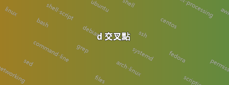
作為練習，我嘗試繪製棱鏡 [0,2] x [0,4] x [0,6] 和平面 x + y + z = 5 的交點。

我的結果是：

\documentclass{article}

\usepackage{pgfplots}
\pgfplotsset{compat=newest}

\begin{document}
    
\begin{tikzpicture}[x={(-0.45cm,-0.385cm)},y={(1cm,-0.1cm)},z={(0,1cm)}]
    \draw [->] (0,0,0) -- (6,0,0) node [below left] {$x$};
    \draw [->] (0,0,0) -- (0,6,0) node [right] {$y$};
    \draw [->] (0,0,0) -- (0,0,6) node [right] {$z$};
    
    \filldraw [thick, orange, fill opacity=0.3] (0,0,5) -- (0,4,1) -- (1,4,0) -- (2,3,0) -- (2,0,3) -- cycle;
    \filldraw [thick, blue, fill opacity=0.2] (2,3,0) -- (2,0,3) -- (5,0,0) -- cycle;
    \filldraw [thick, blue, fill opacity=0.2] (1,4,0) -- (0,5,0) -- (0,4,1) -- cycle;
    
    \filldraw [thick, orange, fill opacity=0.3] (2,3,0) -- (2,0,0) -- (2,0,3) -- cycle;
    \filldraw [thick, orange, fill opacity=0.3] (1,4,0) -- (0,4,0) -- (0,4,1) --cycle;
    
\end{tikzpicture}

\end{document}

我現在有一些問題：

• 我認為有很多程式碼只是為了將一個簡單的數學體積表示為 [0,2] x [0,4] x [0,6]。有沒有更有效的繪製方法？
• 我需要手動計算交集然後表示它嗎？或是有什麼直接的方法嗎？
• 如何透過使用axis環境和\addplot命令而不是獲得相同的結果\draw？我已經嘗試過，但我是新手\addplot3，我在軸位置（view={}{}）方面遇到了麻煩colormap，沒有均勻的顏色，表面有一個網格，很難理解圖片，我對交叉點也有同樣的疑問，做我需要手動計算它們嗎？

全棱鏡為：

\draw [fill=orange, fill opacity=0.3] (0,0,6) -- (2,0,6) -- (2,4,6) -- (0,4,6) -- cycle ;
\draw [fill=orange, fill opacity=0.3] (2,0,0) -- (2,0,6) -- (2,4,6) -- (2,4,0) -- cycle ;
\draw [fill=orange, fill opacity=0.3] (2,4,0) -- (0,4,0) -- (0,4,6) -- (2,4,6) -- cycle ;

Answer 1

無論您做什麼，請考慮以更系統化的方式安裝 3D 視圖。要實現這一點的最佳方法也許是使用asymptote，它確實有計算 3d 相交的工具。如果你想用pgfplots，就用patch plots。但是，為此您仍然需要自己計算交集。這篇文章要提到一些實驗鈦kZ庫它還允許人們計算 3d 中的交點。

\documentclass{article}
\usepackage{tikz}
\usetikzlibrary{3dtools}%https://github.com/marmotghost/tikz-3dtools
\begin{document}
\pgfdeclarelayer{background} 
\pgfdeclarelayer{foreground}
\pgfdeclarelayer{behind}  
\pgfsetlayers{behind,background,main,foreground}   
\begin{tikzpicture}[>=stealth,
    3d/install view={theta=70,phi=110},
    line cap=round,line join=round,
    visible/.style={draw,thick,solid},
    hidden/.style={draw,very thin,cheating dash},
    3d/polyhedron/.cd,fore/.style={visible,fill opacity=0.6},
    back/.style={fill opacity=0.6,hidden,3d/polyhedron/complete dashes},
    fore layer=foreground,
    back layer=background
    ]
  \draw [->] (0,0,0) coordinate (O) -- (6,0,0) coordinate (ex) node [below left] {$x$};
  \draw [->] (0,0,0) -- (0,6,0) coordinate (ey) node [right] {$y$};
  \draw [->] (0,0,0) -- (0,0,6) coordinate (ez) node [right] {$z$};
  \path (5,0,0) coordinate (A) (0,5,0) coordinate (B) (0,0,5) coordinate (C)
   (2.5,0,0) coordinate (a) (0,3.5,0) coordinate (b) (0,0,2) coordinate (c) ;
  \path[3d/.cd,plane with normal={(ex) through (a) named px},
      plane with normal={(ey) through (b) named py},
      line through={(A) and (B) named lAB},
      line through={(A) and (C) named lAC},
      line through={(B) and (C) named lBC}];
  \path[3d/intersection of={lAB with px}] coordinate (pABx)
   [3d/intersection of={lAB with py}] coordinate (pABy)
   [3d/intersection of={lAC with px}] coordinate (pACx)
   [3d/intersection of={lBC with py}] coordinate (pBCy);
  \pgfmathsetmacro{\mybarycenterA}{barycenter("(A),(pABx),(pACx),(a)")} 
  \pgfmathsetmacro{\mybarycenterB}{barycenter("(B),(pABy),(pBCy),(b)")} 
  \tikzset{3d/polyhedron/.cd,O={(\mybarycenterA)},color=blue,
      draw face with corners={{(A)},{(pABx)},{(pACx)}},
      draw face with corners={{(A)},{(pABx)},{(a)}},
      draw face with corners={{(A)},{(a)},{(pACx)}},
      O={(\mybarycenterB)},
      draw face with corners={{(B)},{(pABy)},{(pBCy)}},
      draw face with corners={{(B)},{(pABy)},{(b)}},
      draw face with corners={{(B)},{(b)},{(pBCy)}},
      color=orange,O={(1,1,1)},
      draw face with corners={{(pABx)},{(pACx)},{(C)},{(pBCy)},{(pABy)}},
      draw face with corners={{(a)},{(pACx)},{(C)},{(O)}},
      draw face with corners={{(b)},{(pBCy)},{(C)},{(O)}},
      draw face with corners={{(b)},{(pABy)},{(pABx)},{(a)},{(O)}}
      }
\end{tikzpicture}
\end{document}

還是很多努力的。然而，有一個好處：您可以更改視圖並仍然獲得正確的結果。例如3d/install view={theta=70,phi=60},你會得到

asymptote當然，對於和解決方案也是如此patch plot（也許除了自動將隱藏線虛線化的可能性之外）。