


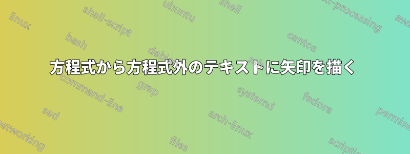
方程式内のボックスから方程式の外側のテキストの
特定の部分 (たとえば、記号) に矢印を描画したいと思います。 矢印はテキストを通過してはいけません。=
私のコード:
\documentclass[
    pdftex,a4paper,11pt,oneside,fleqn,
    bibliography=totoc,listof=totoc,
    headlines=2.1,headsepline,
    numbers=noenddot
]{scrreprt}


%%%----- Mathe ----------------------------------
\usepackage{amsmath,amsfonts,amssymb,bm}
\usepackage[squaren,textstyle]{SIunits}
\usepackage{icomma}

\usepackage{mathtools}
\usepackage[makeroom]{cancel}
\usepackage{trfsigns}


%%% ------ Formel schöner darstellen ------------
\usepackage{tcolorbox}
\tcbuselibrary{listings,theorems}
\def\mathunderline#1#2{\color{#1}\underline{{\color{black}#2}}\color{black}}

%%%--------------------------------------------------------
%%%----- Beginn Dokument ----------------------------------
\begin{document}

    \begin{equation}
\tcbset{fonttitle=\scriptsize}
 \begin{split}
    \sigma_{\mathrm{n}} &= \sigma_{\mathrm{n}, \nu = 1} + \sigma_{\mathrm{n}, \nu = 1, \mu = 1} + \sigma_{\mathrm{n}, \mu = 1}\\
    &= \Bigg( \dfrac{\hat{B}_{\delta \mathrm{s}, \nu = 1}^{2} + \hat{B}_{\delta \mathrm{r}, \mu = 1}^{2}}{4 \cdot \mu_{0}} + \dfrac{\hat{B}_{\delta \mathrm{s}, \nu = 1} \cdot \hat{B}_{\delta \mathrm{r}, \mu = 1}}{2 \cdot \mu_{0}} \Bigg) \cdot \Big( 1 + \cos \left(2 p \alpha - 2 \omega_{\mathrm{el}} t \right) \Big)\\
    &= \dfrac{\hat{B}_{\delta \mathrm{s}, \nu = 1}^{2} + \hat{B}_{\delta \mathrm{r}, \mu = 1}^{2} + 2 \cdot \hat{B}_{\delta \mathrm{s}, \nu = 1} \cdot \hat{B}_{\delta \mathrm{r}, \mu = 1}}{4 \cdot \mu_{0}} \cdot \Big( 1 + \cos \left(2 p \alpha - 2 \omega_{\mathrm{el}} t \right) \Big)\\
    &= \dfrac{\left( \hat{B}_{\delta \mathrm{s}, \nu = 1} + \hat{B}_{\delta \mathrm{r}, \mu = 1} \right)^{2}}{4 \cdot \mu_{0}} \cdot \Big( 1 + \cos \big(2 p \alpha - \tcboxmath[boxsep=1pt,left=2pt,right=2pt,top=1pt,bottom=1pt, colback=white,colframe=red]{2 \omega_{\mathrm{el}}} \, t \big) \Big) \, \text{.}
 \end{split}
 \label{eq: Radialkraftwelle_Grundwelle}
\end{equation}

Das Ergebnis für das Grundwellen-Luftspaltfeld ist eine Radialkraftwelle, die sich mit einer Frequenz von $f_{\mathrm{h}} = 2f_{\mathrm{el}}$ (1. Hauptordnung) ausbreitet.

\end{document}
望ましい結果:

答え1
tikzmarksこれを実現するには、Tiのライブラリとして使用できます。けZ は、これを機能させるためにいずれにしても必要となるskinsライブラリをロードすると自動的にロードされます。このライブラリを使用すると、テキスト内にマークまたはノードを配置し、オプション を持つを使用してこれらのマークとノードを参照できます。たとえば、テキスト内に を配置すると、後で などを使用してこのノードに線を引くことができます。この手法を使用すると、方程式の から下のテキスト内の式の関連部分に矢印を描くことができます。tcolorboxtikzpictureremember picture, overlay\tikzmarknode{mynode}{some text}\tikz \draw (mynode) -- +(0,1);\tcboxmath
を参照できるようにするには\tcboxmath、オプション を追加する必要があります。enhanced, remember as=[name]このオプションは、ライブラリを事前にロードした場合にのみ使用できますskins。
矢印がページ上のテキストの周囲を回るには、パッケージを使用してtikzpagenodes右のテキスト余白を参照します。便宜上、矢印の位置合わせを容易にする座標をいくつか作成しました。
\documentclass[
    pdftex,a4paper,11pt,oneside,fleqn,
    bibliography=totoc,listof=totoc,
    headlines=2.1,headsepline,
    numbers=noenddot
]{scrreprt}

%%%----- Mathe ----------------------------------
\usepackage{amsmath,amsfonts,amssymb,bm}
\usepackage[squaren,textstyle]{SIunits}
\usepackage{icomma}

\usepackage{mathtools}
\usepackage[makeroom]{cancel}
\usepackage{trfsigns}

%%% ------ Formel schöner darstellen ------------
\usepackage{tcolorbox}
\tcbuselibrary{listings,theorems,skins}
\def\mathunderline#1#2{\color{#1}\underline{{\color{black}#2}}\color{black}}

\usepackage{tikzpagenodes}
\usetikzlibrary{tikzmark}

%%%--------------------------------------------------------
%%%----- Beginn Dokument ----------------------------------
\begin{document}

\begin{equation}
\tcbset{fonttitle=\scriptsize}
 \begin{split}
    \sigma_{\mathrm{n}} &= \sigma_{\mathrm{n}, \nu = 1} + \sigma_{\mathrm{n}, \nu = 1, \mu = 1} + \sigma_{\mathrm{n}, \mu = 1}\\
    &= \Bigg( \dfrac{\hat{B}_{\delta \mathrm{s}, \nu = 1}^{2} + \hat{B}_{\delta \mathrm{r}, \mu = 1}^{2}}{4 \cdot \mu_{0}} + \dfrac{\hat{B}_{\delta \mathrm{s}, \nu = 1} \cdot \hat{B}_{\delta \mathrm{r}, \mu = 1}}{2 \cdot \mu_{0}} \Bigg) \cdot \Big( 1 + \cos \left(2 p \alpha - 2 \omega_{\mathrm{el}} t \right) \Big)\\
    &= \dfrac{\hat{B}_{\delta \mathrm{s}, \nu = 1}^{2} + \hat{B}_{\delta \mathrm{r}, \mu = 1}^{2} + 2 \cdot \hat{B}_{\delta \mathrm{s}, \nu = 1} \cdot \hat{B}_{\delta \mathrm{r}, \mu = 1}}{4 \cdot \mu_{0}} \cdot \Big( 1 + \cos \left(2 p \alpha - 2 \omega_{\mathrm{el}} t \right) \Big)\\
    &= \dfrac{\left( \hat{B}_{\delta \mathrm{s}, \nu = 1} + \hat{B}_{\delta \mathrm{r}, \mu = 1} \right)^{2}}{4 \cdot \mu_{0}} \cdot \Big( 1 + \cos \big(2 p \alpha - \tcboxmath[enhanced,remember as=from,boxsep=1pt,left=2pt,right=2pt,top=1pt,bottom=1pt,colback=white,colframe=red,]{2 \omega_{\mathrm{el}}} \, t \big) \Big) \, \text{.}
 \end{split}
 \label{eq:Radialkraftwelle_Grundwelle}
\end{equation}

Das Ergebnis für das Grundwellen-Luftspaltfeld ist eine Radialkraftwelle, die sich mit einer Frequenz von $f_{\mathrm{h}} = \tikzmarknode{to}{2f_{\mathrm{el}}}$ (1. Hauptordnung) ausbreitet.

\begin{tikzpicture}[overlay, remember picture]
    \coordinate (south of from) at ([yshift=-0.25cm]from.south);
    \coordinate (south of to) at ([yshift=-0.25cm]to.south);
    \coordinate (text margin right) at ([xshift=0.5cm]current page text area.east);
    \draw[thick, red, -stealth, rounded corners=2.5pt] (from.south) -- (south of from) --
    (south of from -| text margin right) -- (south of to -| text margin right) -- (south of to) -- (to.south);
\end{tikzpicture}

\end{document}
